Choosing a Voltage Divider Resistor for a Light Dependent Resistor

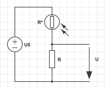
Imagine that you are planning to use a Light Dependent Resistor (LDR) for your new IoT prototype in order to detect whether or not a lamp is turned on in a (otherwise dark) room. A common way to solve this problem is the usage of a voltage divider circuit in the following form:

In this blog post, we will discuss how to choose the voltage divider’s resistances appropriately.

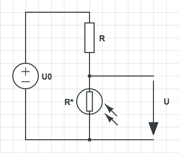
In the above diagram, the LDR is denoted as \(R^*\), and \(R\) is another resistance required to divide the compliance voltage \(U_0\). Depending on the light that falls onto the LDR, the resistance of \(R^*\) and the voltage \(U\) change. The voltage \(U\) can be converted into a discrete value using an Analog-to-Digital-Converter (ADC), and the retrieved value can then be evaluated in a micro-controller (μC) program to determine the current lighting conditions in the room. In the above diagram, if the light is very bright, \(U\) would be large (close to \(U_0\)). If no light falls onto the LDR (in a dark room), the voltage \(U\) will tend towards small values. If you want to achieve the opposite behavior (small value of \(U\) for bright light), you can swap the resistor \(R\) with the LDR. This is illustrated in the figure below:

However, there is one major problem when using a voltage divider: Typically, one would like \(U\) to cover a wide range of values, ideally between 0V and \(U_0\) (\(U \in [0V, U_0]\)), independently of the range of \(R^*\). This is, for example, important when ADCs are used since an ADC only has a limited resolution. If \(U\) only changes in a small range for different lighting conditions, then we do not have a sufficient signal-to-noise ratio, and it will become very difficult to distinguish bright from dark. Let us assume, for example, that in our configuration (first diagram, with \(U_0\) = 5V), the voltage \(U\) varies between 3.5V (very dark) and 4.5V (very bright). If we are now using an 8-bit ADC (assuming that the reference voltage of the ADC is also \(U_0\)), we have a voltage resolution of \(5V/256\), which is approx. \(0.02V\). But since the input voltage only moves around in the interval \([3.5V, 4.5V]\), the ADC will only generate an interval of about \(1V/0.02V=50\) distinguishable values, although 256 would be theoretically possible. Taking slightly changing lighting conditions and other noise sources into account, this interval containing 50 discrete values is rather small. It will most likely lead to false assertions about the state of the lamp (on/off) in the room. Even if we use high-resolution ADCs in this configuration, we will run into problems if we have significant noise in \(U\). Hence, we should ensure that the interval of values \(U\) covers is as large as possible to maximize the signal-to-noise ratio.

The good news is that we can maximize the range of \(U\) by selecting \(R\) appropriately if we know our extreme values (e.g., for dark and bright) of \(R^*\). The bad news is: If the ratio between these extreme values – which are given by the physical constraints of the LDR (or some other component) and its environment and which cannot be chosen by us – is too small, then we again run into the problem that \(U\) will only cover a small interval. For this reason, you should ensure that the varying resistor (LDR, force-sensitive resistor, etc.) you use has a high ratio between the extreme values for those conditions you want to distinguish.

Step-by-step guide

1. Based on the previous remarks, you should follow these steps for the setup of a suitable voltage divider:
2. Select a varying resistance (e.g., LDR) suitable for your task
3. Choose either of the above circuit diagrams (whichever suits your needs)
4. Measure the minimum and maximum values for R^* for the extreme conditions of your environment
5. Compute the ratio \(R^*_{max} / R^*_{min}\) for the extreme values of \(R^*\). If the ratio is too small, return to 1. and find another component. If you are unsure if your ratio is fine, you can continue with the following steps and conduct some experiments afterward.
6. Choose \(R=\sqrt{R^*_{min} \cdot R^*_{max}}\). This guarantees that you cover the largest interval for \(U\) (if you are interested in why, you can continue reading the following section).
7. Build your circuit and test your setup to ensure that it is sufficiently robust. If you encounter problems, you either have to start with step one again or experiment with more advanced algorithmic approaches (outside the scope of this article).

If you realize that the minimum value of \(R^*\) is close to 0Ω (which is rarely the case), then you should be doing fine with a value of R between 500Ω and 1000Ω. If possible, you should ensure that \(R^*_{min}+R > 500 \Omega\), to avoid too large currents.

Maximizing the Voltage Margin for a Voltage Divider

We assume that both \(R^*_{max}\) and \(R^*_{min}\) are known. \(U_0\) is typically also known in advance. However, we will see that it does not play a role in calculating \(R\). For a certain resistance \(R^* \in [R^*_{min}, R^*_{max}]\) we know that (following Fig. 1):

\[\begin{align} U(R)=U_0 \frac{R}{R^* + R} \end{align}\]

Since we wish to maximize the voltage margin for \(U\), we introduce a new quantity \(\Delta U\), which is simply the difference of the voltage \(U\) for the extreme values of \(R^*\):

\[\begin{align*} \Delta U(R) &= U_{max}(R) - U_{min}(R) \\ &= U_0 \frac{R}{R^*_{min} + R} - U_0 \frac{R}{R^*_{max} + R} \\ &= U_0 \Bigg[\frac{R}{R^*_{min} + R} - \frac{R}{R^*_{max} + R} \Bigg] \\ &= U_0 \Bigg[\frac{R(R^*_{max} + R) - R(R^*_{min} + R)}{(R^*_{min} + R)(R^*_{max} + R)} \Bigg] \\ &= U_0 \Bigg[\frac{R(R^*_{max} - R^*_{min})}{(R^*_{min} + R)(R^*_{max} + R)} \Bigg] \\ \end{align*}\]

In order to maximize above function \(\Delta U(R)\) we first compute the derivative \(\frac{\partial}{\partial R} \Delta U\):

\[\begin{align*} \frac{\partial}{\partial R} \Delta U &= U_0\Bigg[\frac{(R^*_{max} - R^*_{min})(R^*_{min} + R)(R^*_{max} + R)-(R^*_{max} - R^*_{min})(R^*_{min} + R^*_{max} + 2R)}{(R^*_{min} + R)^2(R^*_{max} + R)^2}\Bigg] \\ &= U_0\Bigg[\frac{(R^*_{min} - R^*_{max})\big[R(R^*_{min} + R^*_{max} + 2R)- (R^*_{min} + R)(R^*_{max} + R)\big]}{(R^*_{min} + R)^2(R^*_{max} + R)^2}\Bigg] \\ &= U_0\Bigg[\frac{(R^*_{min} - R^*_{max})\big[2R^2-R^*_{min}R^*_{max} - R^2\big]}{(R^*_{min} + R)^2(R^*_{max} + R)^2}\Bigg] \\ &= U_0\Bigg[\frac{(R^*_{min} - R^*_{max})\big[R^2-R^*_{min}R^*_{max}\big]}{(R^*_{min} + R)^2(R^*_{max} + R)^2}\Bigg] \end{align*}\]

Then, we solve \(\frac{\partial \Delta U}{\partial R} = 0\), in order to detect the extrema of the function:

\[\begin{align*} 0 &= \frac{\partial}{\partial R}\Delta U \\ 0 &= U_0\Bigg[\frac{(R^*_{min} - R^*_{max})\big[R^2-R^*_{min}R^*_{max}\big]}{(R^*_{min} + R)^2(R^*_{max} + R)^2}\Bigg] \\ 0 &= (R^*_{min} - R^*_{max})\big[R^2-R^*_{min}R^*_{max}\big] \\ \end{align*}\]

And, since we assume that \(R^*_{max}\) is strictly larger than \(R^*_{min}\), hence \(R^*_{max} > R^*_{min}\), we finally get:

\[\begin{align*} 0 &= R^2-R^*_{min}R^*_{max}\\ R^2 &= R^*_{min}R^*_{max} \\ R &= \sqrt{R^*_{min}R^*_{max}} \\ \end{align*}\]

It is easy to see that above solution for \(R\) maximizes the voltage margin.

Example

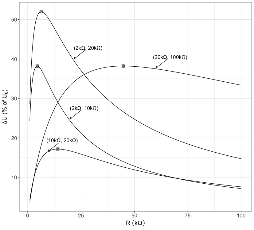
In the figure below we show the behaviour of the voltage margin for different min-max value pairs of \(R^*\).

As we can see from the diagram, for \(R^*_{min}=2k\Omega\) and \(R^*_{max}=10k\Omega\), we can – in the best case – achieve a voltage margin that covers about 38% of the original range of \(U_0\). If we read off the corresponding value of \(R\) from the abscissa, we have approx. \(R=5k\Omega\). The true value is \(R=\sqrt{2k\Omega \cdot 10k\Omega}\approx 4.5k\Omega\).

As we mentioned before, not the difference \(R^*_{max} - R^*_{min}\) is important for the max. voltage margin, but rather the ratio \(R^*_{max}/R^*_{min}\). For example, the value pair \((R^*_{min}, R^*_{max})= (10k\Omega, 20k\Omega)\) has a larger difference \(R^*_{max}-R^*_{min}\) than \((R^*_{min}, R^*_{max})= (2k\Omega, 10k\Omega)\), however, the max. voltage margin is significantly lower for \((10k\Omega, 20k\Omega)\). If we have \((R^*_{min}, R^*_{max})= (20k\Omega, 100k\Omega)\), then the max. voltage margin we can achieve is exactly the same as for \((R^*_{min}, R^*_{max})= (2k\Omega, 10k\Omega)\), since the min-max ratio is equivalent, although both curves differ. In practice, one prefers the setting \((20k\Omega, 100k\Omega)\), because it is not as steep.

To increase the voltage margin, we must find a setting that allows for a higher min-max ratio of \(R^*\). We can see in the figure that if we, for example, double \(R^*_{max}\) for \((R^*_{min}, R^*_{max})= (2k\Omega, 10k\Omega)\), \(\Delta U\) increases by approximately 15%. Nevertheless, only about 53% of the original range of \(U_0\) is covered in this case.

In practice, if one has to find the closest suitable resistor for \(R\), moving towards slightly larger values is usually better. This is because the slope of the voltage margin curve (as seen in the above figure) is not as high when we leave the optimum towards higher values as if we would move towards smaller ones.

The R-Code for generating the above figure is listed in the Jupyter notebook below. You can also exceute the notebook yourself: