Notes on the Runtime Complexity of Latin Hypercube Sampling

\(
\def\myT{\mathsf{T}} \def\myPhi{\mathbf{\Phi}} \)

Recently, I needed to tune several parameters of a simple algorithm (five in total). To efficiently explore the parameter space, I chose to use a Latin Hypercube Sampling (LHS) design. Because each design point could be evaluated very quickly, selecting 1,000 design points seemed reasonable.

In R, the lhs package provides a convenient function, optimumLHS, to generate such designs. However, when attempting to generate (n = 1000) points, the function failed to return even after several minutes. This behavior highlights an important issue: the runtime complexity of the LHS algorithm.

To better understand this, I measured the runtime of LHS for different numbers of design points. The following R code illustrates how these measurements were obtained:

library(lhs)
library(ggplot2)
library(MASS)
library(dplyr)
library(pbapply)

runLHS <- function(whichN, repeats){
  lhsTimes <- data.frame()
  for(i in whichN){
    for(j in 1:repeats) {
      tStart <- proc.time()
      invisible(optimumLHS(n = i, k = 5, verbose = FALSE))
      tt <- (proc.time() - tStart)
      lhsTimes<-rbind(lhsTimes,data.frame(user=tt[1], system=tt[2], elapsed=tt[3], n=i))
    }
  }
  return (lhsTimes)
}


res <- pblapply(X=rev(1:30)*10, FUN=runLHS, 10, cl=1)
res <- do.call(rbind, res)
# saveRDS(object=res, file="lhs.rds") # In case you want to save the results
# res <- readRDS(file="lhs.rds") # In case you want to load the results
stop("Stop here for the moment")

plotData <- res[which(res$elapsed>.01),] # smaller values are not really interesting
p <- ggplot(plotData,aes(x=n,y=user)) + geom_point()
p <- p + theme_bw()
p <- p + ylab("computation time / s") +
  theme(axis.text=element_text(size=12),
        axis.title=element_text(size=14, face="bold"))
plot(p)

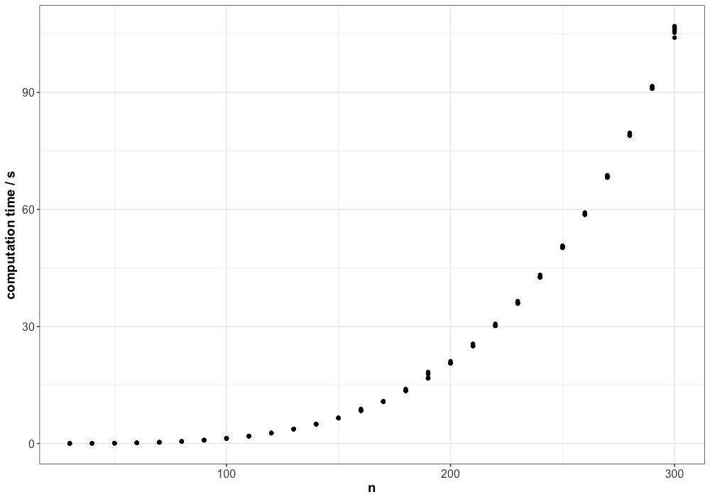
The corresponding plot is shown below:

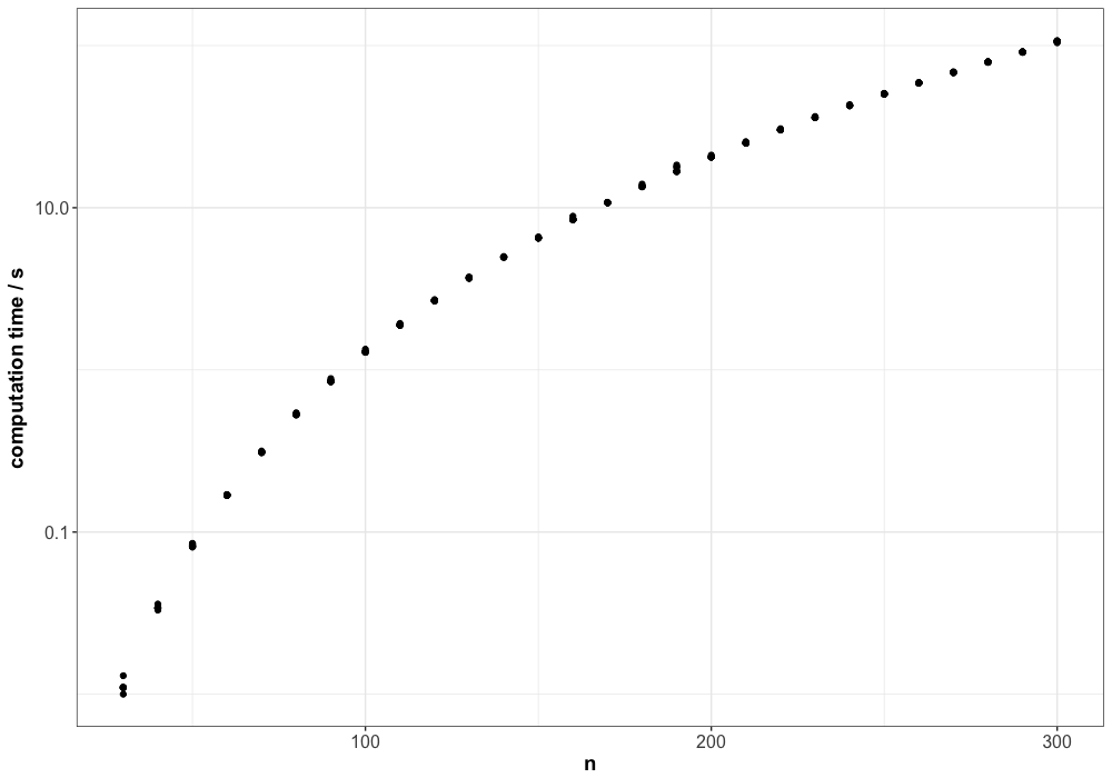
At first glance, the runtime appears to grow at least polynomially, and it could even suggest exponential growth. To investigate this further, we add a logarithmic scale to the y-axis:

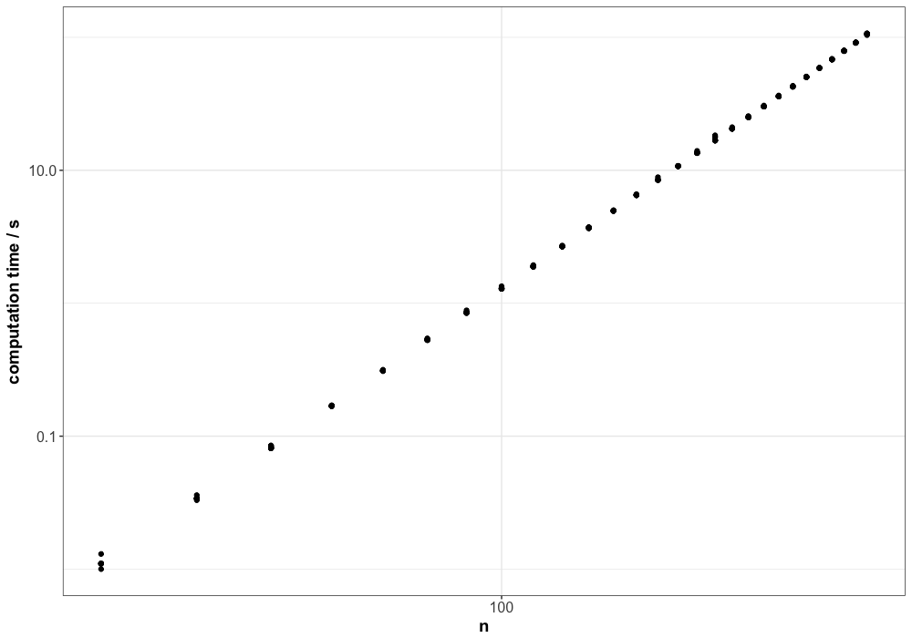
If the runtime were exponential, the log-scaled y-axis would produce a straight line. Since this is not the case, a polynomial growth seems more likely. To confirm, we also apply a log10 scale to the x-axis:

Since we now observe a straight line on the log-log plot, it is reasonable to conclude that the runtime of the LHS algorithm grows polynomially. Next, it is interesting to determine the order of this polynomial. To do so, we estimate the slope and intercept of the line using linear regression.

Because we have 10 measurements for each value of \(n\), we can employ a weighted linear regression approach to account for variations in the observed runtimes.

with

and

The R code for estimating the Intercept \(b\) and the slope \(m\) of the line is as follows:

# Apply log10 to the data
log_n = log10(plotData$n)
log_y = log10(plotData$user)
log_data <- data.frame(log_n, log_y)

#
# Since we repeated each run several times: Measure the variance for each point n
#
grouped <- group_by(cbind(data.frame(log_n=log_n), data.frame(log_y=log_y)), log_n)
stats <- summarise(grouped, mean=mean(log_y), var=var(log_y))

# Now assign the corresponding variance to each data-point again
mergedData <- merge(log_data, stats)

# Prepare the vectors and matrices for the weighted linear least squares estimator
W = diag(1.0 / mergedData$var)
X = cbind(1,mergedData$log_n)
y = mergedData$log_y

# Estimate the Intercept and Slope using weighted linear least squares
theta = ginv(t(X) %*% W %*% X) %*% t(X) %*% W %*% y
cat("slope m=", theta[2], ". Intercept b=", theta[1], sep="")

# Plot the estimated line
p <- ggplot(plotData,aes(x=n,y=user)) +
  geom_point() +
  scale_y_log10() +
  scale_x_log10() +
  geom_abline(slope=theta[2], intercept = theta[1]) +
  theme_bw() +
  ylab("computation time / s") +
  theme(axis.text=element_text(size=12),
        axis.title=element_text(size=14,face="bold"))
plot(p)

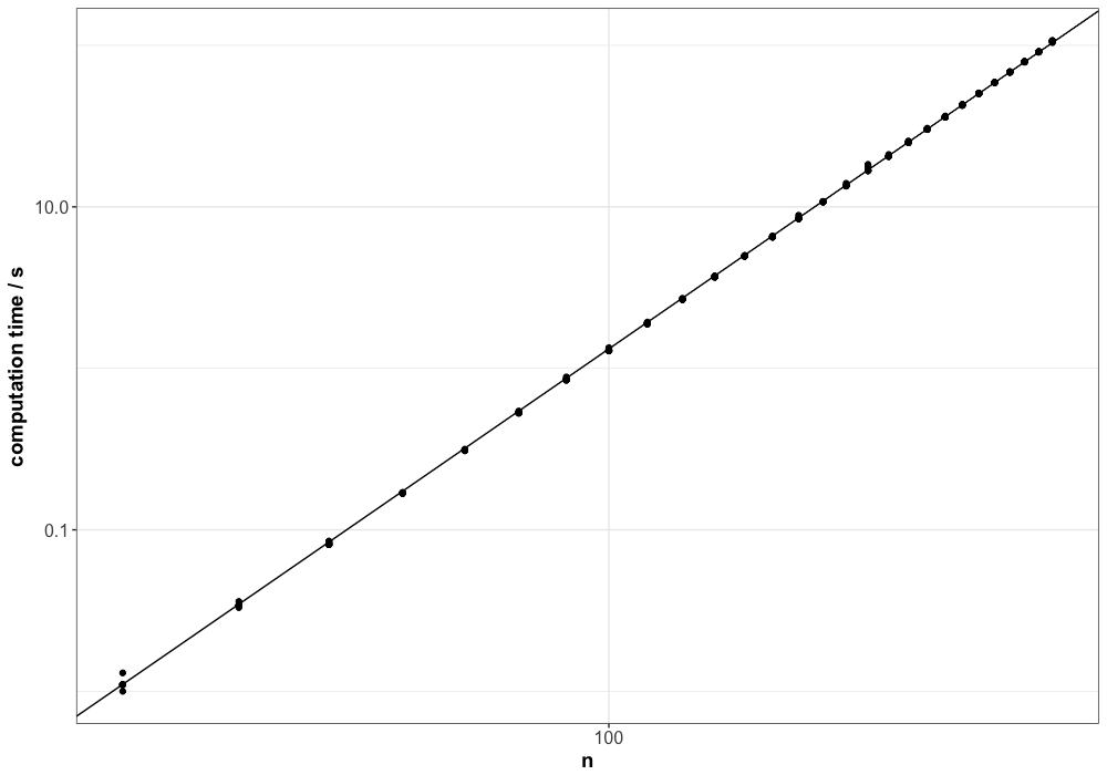
The estimator computes the following values for the slope and the intercept:

Slope m=3.993954. Intercept b=-7.875513

The fitted line aligns closely with the data, as illustrated in the plot below:

Using the estimated slope and intercept, we can now express the expected runtime of the LHS algorithm as a function of the number of design points \(n\):

The estimated runtime from the fitted line is slightly pessimistic, so in practice the actual computation time (at least on my machine) is likely a bit lower. Extrapolating this estimate to \(n=1000\), we would expect a runtime of approximately 16,000 seconds, or about 4.5 hours.

In summary, we can conclude that the LHS algorithm exhibits a runtime complexity of order \(\mathcal{O}(n^4)\).