• Introduction
• Implementation in R
• Example
• Appendix
  • A1: Code
  • A2: Further Examples
    • Example 1
    • Example 2
    • Example 3
    • Example 4

Introduction

Conway’s Game of Life is a so-called zero-player game, developed by British mathematician John Horton Conway in 1970. It begins with an initial configuration set by the player, and from that point on, it evolves automatically without any further interaction.

The rules are quite simple. Here is an excerpt from wikipedia.org:

The universe of the Game of Life is an infinite, two-dimensional orthogonal grid of square cells, each of which is in one of two possible states: alive or dead (or populated and unpopulated, respectively). Every cell interacts with its eight neighbors, which are the cells that are horizontally, vertically, or diagonally adjacent. At each step in time, the following transitions occur:

1. Any live cell with fewer than two live neighbors dies, as if by underpopulation.
2. Any live cell with two or three live neighbors lives on to the next generation.
3. Any live cell with more than three live neighbors dies, as if by overpopulation.
4. Any dead cell with exactly three live neighbors becomes a live cell, as if by reproduction.

The initial pattern constitutes the seed of the system. The first generation is created by applying the above rules simultaneously to every cell in the seed; births and deaths occur simultaneously, and the discrete moment at which this happens is sometimes called a tick. Each generation is a pure function of the preceding one. The rules continue to be applied repeatedly to create further generations.

In this post, we will implement the Game of Life in \(R\) and explore some of the results it produces.

Implementation in R

In principle, the grid in Conway’s Game of Life is infinite. Due to the limitations of our computers, however, we work with a finite grid. For our experiments, we will use relatively small grid sizes.

First, we need a function to initialize the grid. Each cell has a 50% chance of being alive:

randInitWorld <- function(dimX, dimY) {
  matrix(sample(c(TRUE, FALSE), dimX * dimY, replace = TRUE), dimY, dimX)
}

Next, we define a function to count the number of live neighbors for each cell in the grid. For each cell, we look at its surrounding 3×3 box (shrinking the box at the edges) and count the number of live cells—excluding the center cell itself:

countAliveNeighbors <- function(X) {
  d <- dim(X)
  C <- apply(merge(1:d[1], 1:d[2]), 1,
    function(i) {
      sum(X[max(1, i[1] - 1):min(d[1], i[1] + 1),
            max(1, i[2] - 1):min(d[2], i[2] + 1)]) - X[i[1], i[2]]
    }
  )
  matrix(C, d[1], d[2])
}

Now we’re ready to write a function that performs the transition to the next generation. According to the rules, a cell will be alive in the next generation if:

1. It has exactly three live neighbors, or
2. It is currently alive and has exactly two live neighbors.

All other cells will be dead in the next generation. These two simple conditions make it easy to implement the evolution step:

evolveNextGeneration <- function(XWorld) {
  XWorldCount <- countAliveNeighbors(XWorld)
  (XWorldCount == 3) | XWorld & (XWorldCount == 2)
}

And that’s essentially it. We only need a few utility functions to evolve the grid world over multiple time steps and to visualize the grid after each transition. The complete code is available on GitHub and is also included in the appendix.

Example

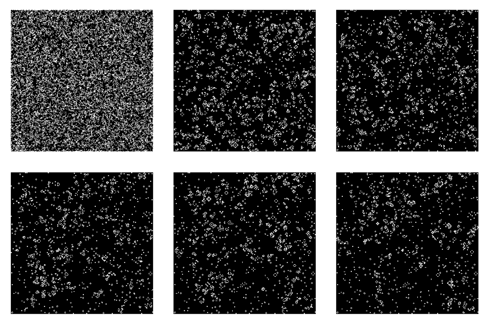
Let’s take a look at how a randomly initialized 100×100 grid evolves over time:

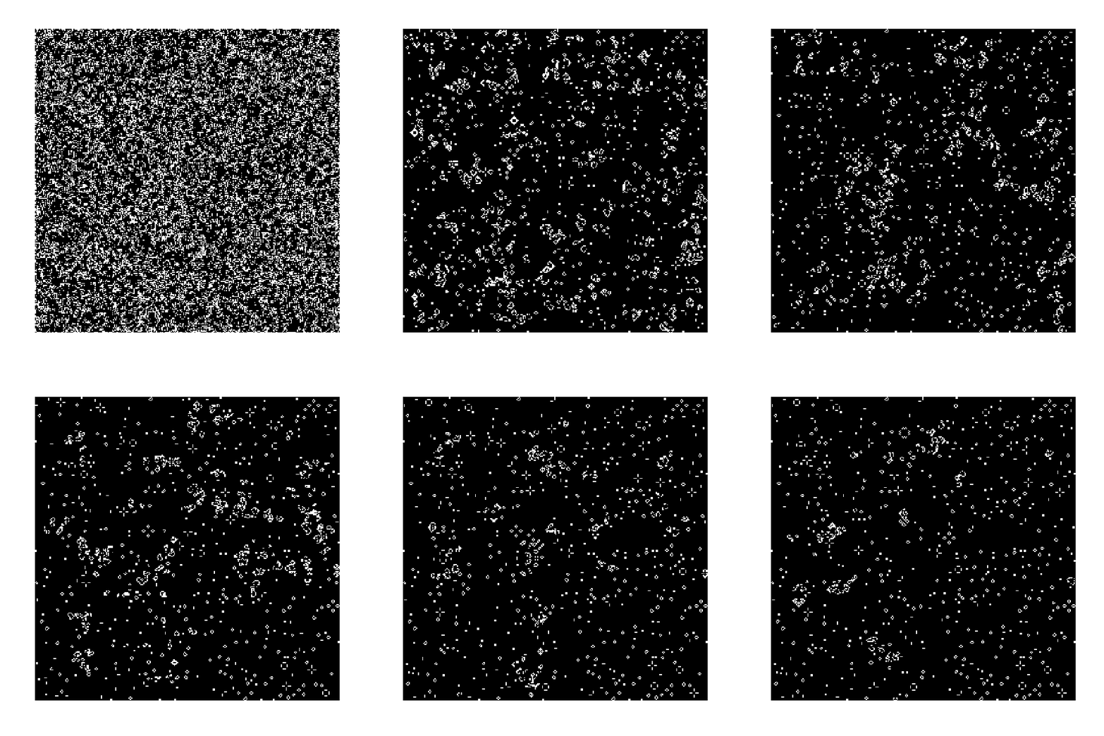
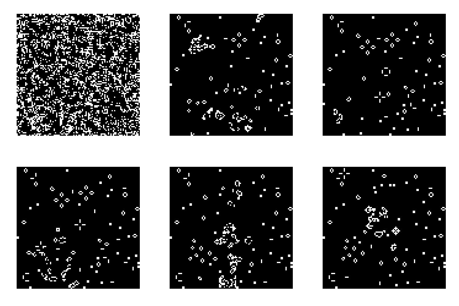
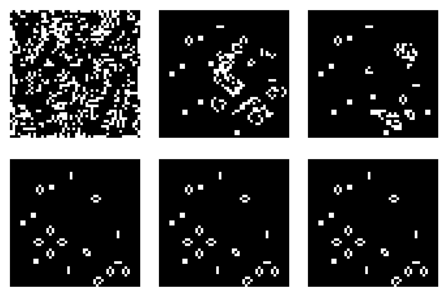
Depending on the initial configuration, many interesting and diverse patterns can emerge. A wide variety of known patterns are documented on wikipedia.org.

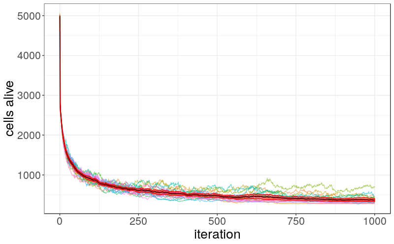
In many cases, the population of live cells never completely dies out but instead stabilizes around a certain number. The following image illustrates how the population evolves over time on a 100×100 grid, based on 20 different random initializations. Initially, about 50% of all cells are alive, but this proportion quickly drops across all runs. After approximately 1,000 iterations, the number of live cells stabilizes at around 350.

Appendix

A1: Code

The GitHub Code is available here!

A2: Further Examples

Example 1

Example 2

Example 3

Example 4