Understanding Bootstrap Sampling: Where Euler’s Number Meets Random Forests

Consider the following classical problem in combinatorics: We have a bowl containing \(n\) distinct balls, each labeled with a unique number. We randomly draw a ball from the bowl, record its number, and then return it to the bowl before the next draw. The order of selection is not relevant, and this process is repeated \(k\) times. This setup is known as sampling with replacement or combinations with repetition.

The number of distinct samples that can be drawn in this way is given by:

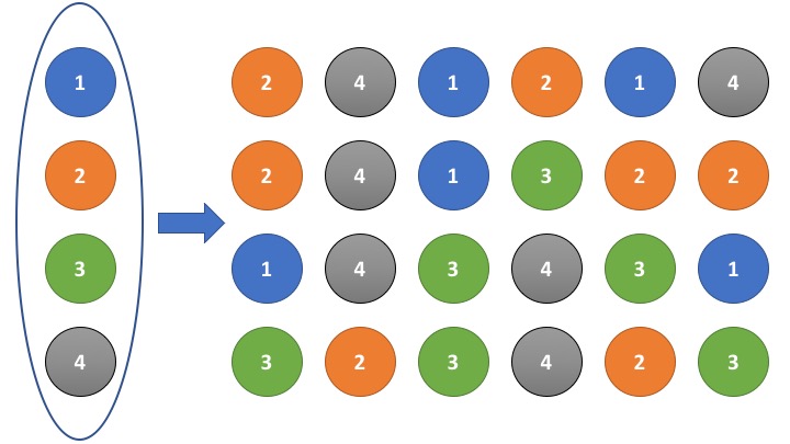
A particularly interesting case arises when \(k = n\), i.e., we draw \(n\) samples from a set of \(n\) unique elements, always replacing the drawn element. The image below illustrates this scenario: on the left is a set of four distinct elements; on the right are several possible samples obtained by sampling \(k = n = 4\) times with replacement. In total, 35 such combinations exist, as determined by the formula above.

Add commentMore actions

But where is Euler’s number in this problem, and what does this have to do with Random Forests, as suggested by the title of this blog post?

I came across this problem while examining the training process of Random Forests (RF) some time ago. Most implementations of Random Forests generate a bootstrap sample for each decision tree by drawing \(n\) times with replacement from the training data, which contains \(n\) examples. This naturally leads to a simple but interesting question: How many unique training examples can we expect in such a sample?

Because the sampling is done with replacement, some examples are likely to appear more than once. Consequently, the probability of obtaining a sample that contains all \(n\) unique elements is relatively low—assuming the training set is sufficiently large. In fact, this probability is precisely:

On the other hand, the probability of drawing a sample containing only a single unique element is even smaller:

Intuitively, one might guess that about 50% of the training examples appear in a typical bootstrap sample. As we’ll see shortly, the actual expected proportion is slightly higher.

To get an initial intuition, we can run a simple simulation in R.

# How often do we want to repeat the simulation?
nSimulations <- 10000

runSimulation <- function(n) {
  # Function that draws a sample of size n from a set of n values
  # and returns the fraction of unique values within the sample
  sampleWithRep <- function(n) {
    # sample the set n times with replacement
    p <- sample(1:n, n, replace = T)

    # compute the fraction of unique values in this sample
    length(unique(p)) / n
  }

  # Run simulation many times and print the mean value for the
  # fraction of unique values within all simulated samples
  mean(sapply(rep(n,nSimulations), sampleWithRep))
}

# Sufficiently large set
n <- 10000

cat("On average, each sample contained", (runSimulation(n) * 100.0),
    "% of the values of the original set.")

The above R-script should give you a value of approx. 63%, which indicates, that (for a sufficiently large training set, e.g. \(n=10\,000\)) roughly around 2/3 of the original training examples will appear in the sample. To show that this value of around 63% actually converges for increasing \(n\), we can run the following code (using the function defined above):

require(ggplot2)
require(scales) # For nicer axis labels

# Number of simulations for each value of n
nSimulations <- 10000

# generate sequence 1, 2, ..., 9, 10, 20, ..., 90, 100, 200, ..., 900, 1000, ..., 90 000
Ns <- c(t(1:9) %o% 10^(0:4))

# Run simulation for different n's
frac <- unlist(mclapply(Ns, runSimulation, mc.cores = 23))

# Zip
result <- data.frame(n = Ns, frac = frac)

# Average of the last 10 values, for convergence line
convergeVal <- round(mean(frac[(length(frac) - 10):length(frac)]), 4)

p <- ggplot(data = result, aes(x = n, y = frac)) +
  geom_line() +
  geom_point(size=2.5) +
  scale_x_log10(breaks = 10^(1:5), labels = comma, limits=c(1,1.2e5)) +
  scale_y_continuous(breaks=c(1, 0.9, 0.8, 0.7, convergeVal), labels = comma) +
  ylab("fraction of unique values") +
  theme_bw() +
  theme(axis.text=element_text(size=20),
        axis.title=element_text(size=20,face="bold"))
plot(p)

The equivalent code in Python would look like this:

import numpy as np
import matplotlib.pyplot as plt

# Number of simulations per value of n
n_simulations = 10_000 # takes some time, reduce to 100 for a fast run

def run_simulation(n: int) -> float:
    """
    Draw n samples with replacement from a set of size n,
    repeated n_simulations times, and return the average fraction
    of unique elements per sample.
    """
    fractions = []
    for _ in range(n_simulations):
        sample = np.random.choice(n, size=n, replace=True)
        unique_fraction = len(np.unique(sample)) / n
        fractions.append(unique_fraction)
    return np.mean(fractions)

# Create values of n: 1–9, 10, 20, ..., 90, 100, 200, ..., 90_000
Ns = np.unique(np.concatenate([np.arange(1, 10) * 10**e for e in range(5)]))

# Run simulations
fractions = [run_simulation(n) for n in Ns]

# Estimate convergence value from last 10 results
convergence_value = np.round(np.mean(fractions[-10:]), 4)

# Plot results
plt.figure(figsize=(10, 6))
plt.plot(Ns, fractions, marker='o', linestyle='-')
plt.xscale('log')
plt.xlabel("n (log scale)", fontsize=14)
plt.ylabel("Fraction of unique values", fontsize=14)
plt.title("Convergence of Unique Sample Fraction in Bootstrap Sampling", fontsize=16)
plt.axhline(convergence_value, color='gray', linestyle='--', label=f'Converges to ~{convergence_value}')
plt.legend()
plt.grid(True, which="both", ls="--", linewidth=0.5)
plt.tight_layout()
plt.show()

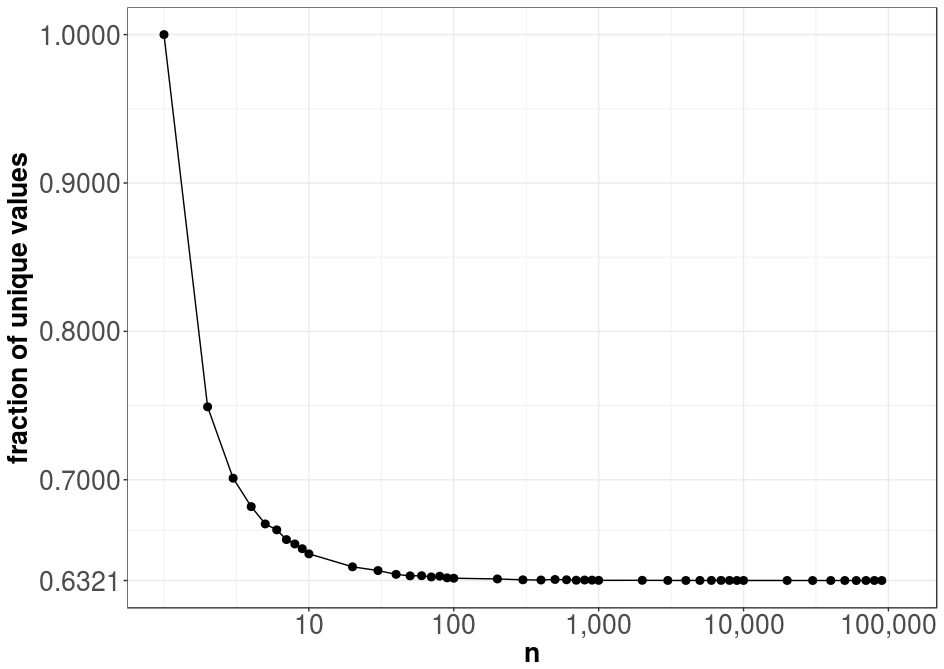
Note that I run the code on a multicore system, since the computation on a single core would require a lot of time. The result of the above code is shown in the following graph:

Add commentMore actions

Obviously, for a training set and sample size of \(n=1\), we always have one unique value in the sample—i.e., 100% uniqueness. As \(n\) increases, the expected fraction of unique elements in the sample converges to approximately 0.6321, a value that might look familiar from various fields such as physics or probability theory. We will soon uncover the origin of this constant.

After performing the simulations, we can now analytically calculate the expected number of unique examples in a sample drawn with replacement. Consider the random variable \(X_i\) for each example \(i \in \{1, \ldots, n\}\), defined as:

• \(X_i = 1\) if example \(i\) is selected at least once,
• \(X_i = 0\) otherwise.

The probability \(P(X_i=1)\) is given by:

It is easier to calculate \(P(X_i=0)\), the probability that example \(i\) is not selected in any of the \(n\) draws. Since each draw has probability \(\frac{n-1}{n}\) of avoiding \(i\), we have:

Therefore, the probability \(P(X_i=1)\) becomes:

As \(n\) approaches infinity, this limit converges to:

This result explains why Random Forests leave out roughly \(\frac{1}{e} \approx 36.8\%\) of the training examples in each bootstrap sample. These omitted samples form the so-called out-of-bag (OOB) data, which can be used as an unbiased estimate of the model’s generalization error.