Constructing a Linear Classifier from Known Decision-Boundary Points
- A Hyperplane Through n Affinely Independent Points
- From the Parametric Form to a Normal Vector
- Signed Distances and the Hesse Normal Form
- Choosing the Orientation and Classifying
- Fitting Noisy Boundary Estimates
- Limitations and the Complete Procedure
- Related Work
- A Synthetic Application: Calibrating a Light-Triggered Relay
- A Runnable Python Example
- References
Suppose we have data points \(\vec x_k \in \mathbb{R}^n\) belonging to two classes. Some points have known class labels, and the remaining points need to be classified. In addition, we have a set of points known to lie on, or close to, the decision boundary. Such boundary estimates might come from domain knowledge or experiments that locate a transition between the two classes.
If an affine hyperplane is a reasonable approximation to the decision boundary, we can construct it from the boundary points and use the labeled observations to identify the class on each side. We first derive the exact construction from \(n\) boundary points, then extend it to fit a hyperplane to a larger set of noisy boundary estimates.

The filled orange circles and blue crosses represent the two known classes. The hollow circles are unlabeled observations, and the gray stars are estimated boundary points. The gray line illustrates a possible linear decision boundary. Some labeled observations lie on the opposite side from most members of their class, so we should not expect perfect separation.
A Hyperplane Through n Affinely Independent Points
To construct an exact hyperplane, we need \(n\) affinely independent points \(\vec p_1,\ldots,\vec p_n \in \mathbb{R}^n\). This means that the \(n-1\) difference vectors
\[\vec p_1-\vec p_2,\ldots,\vec p_1-\vec p_n\]are linearly independent. The condition concerns these differences, not the position vectors themselves. For example, \((0,0)\) and \((1,0)\) determine a unique line even though their position vectors are linearly dependent. If the difference vectors are dependent, the points lie in a lower-dimensional affine subspace and do not determine a unique hyperplane.
Let us start with two distinct points in two dimensions. The line through them has the parametric form
\[\vec x=\vec p_1+t(\vec p_1-\vec p_2),\qquad t\in\mathbb{R}.\]
Here, \(\vec p_1\) is an anchor point and \(\vec p_1-\vec p_2\) is a direction vector. In three dimensions, three noncollinear points similarly define the plane
\[\vec x=\vec p_1+t(\vec p_1-\vec p_2)+s(\vec p_1-\vec p_3), \qquad t,s\in\mathbb{R}.\]For \(n\) affinely independent points in \(\mathbb{R}^n\), the corresponding hyperplane is
\[\begin{equation} \vec x=\vec p_1+\sum_{i=2}^{n}t_i(\vec p_1-\vec p_i), \qquad t_i\in\mathbb{R}. \label{eq:parametricPlane} \end{equation}\]From the Parametric Form to a Normal Vector
The parametric form describes all points on the hyperplane. For classification, however, it is more convenient to use an equation of the form
\[\vec w^{\top}\vec x+b=0,\]where \(\vec w\in\mathbb{R}^n\) is a nonzero normal vector and \(b\in\mathbb{R}\) is an intercept. This is the form of the decision boundary used by linear classifiers, including logistic regression. Knowing the boundary determines these coefficients only up to a nonzero common factor; it does not determine logistic-regression probabilities.
To obtain this form, we need a normal vector orthogonal to every direction vector in equation $\eqref{eq:parametricPlane}$. Arrange the direction vectors as the rows of a matrix:
\[\mathbf A= \begin{pmatrix} (\vec p_1-\vec p_2)^{\top}\\ \vdots\\ (\vec p_1-\vec p_n)^{\top} \end{pmatrix} \in\mathbb{R}^{(n-1)\times n}.\]A normal vector is any nonzero solution of \(\mathbf A\vec n=\vec 0\). Since affine independence gives \(\operatorname{rank}(\mathbf A)=n-1\), the null space is one-dimensional. We normalize a solution to obtain
\[\vec n_0=\frac{\vec n}{\lVert\vec n\rVert_2},\qquad \lVert\vec n_0\rVert_2=1.\]In three dimensions, a cross product of the two direction vectors gives a normal. A generalized cross product extends this construction to \(n-1\) direction vectors in \(\mathbb{R}^n\). For numerical computation, we can instead obtain the null space using a singular value decomposition (SVD). With the full decomposition \(\mathbf A=\mathbf U\mathbf\Sigma\mathbf V^{\top}\), the last column of the \(n\times n\) matrix \(\mathbf V\) is a unit normal. A reduced decomposition can omit that null-space vector, so we need the full set of right singular vectors here.
Taking the inner product of equation $\eqref{eq:parametricPlane}$ with \(\vec n_0\) eliminates every direction term:
\[\begin{align} \vec n_0^{\top}(\vec x-\vec p_1) &=\sum_{i=2}^{n}t_i\underbrace{\vec n_0^{\top}(\vec p_1-\vec p_i)}_{=0} \nonumber \\ &=0. \end{align}\]Therefore, the desired coefficients are simply
\[\begin{equation} \vec w=\vec n_0,\qquad b=-\vec n_0^{\top}\vec p_1. \label{eq:classifierWeights} \end{equation}\]Signed Distances and the Hesse Normal Form
There is also a useful geometric interpretation. Define the signed offset \(d=\vec n_0^{\top}\vec p_1\). The hyperplane equation becomes
\[\begin{equation} \vec n_0^{\top}\vec x=d. \label{eq:hesse} \end{equation}\]
The point with position vector \(d\vec n_0\) is the perpendicular projection of the origin onto the hyperplane. The figure illustrates \(d>0\), but \(d\) can also be negative or zero. Because the normal has unit length, the ordinary distance from the origin to the hyperplane is \(\lvert d\rvert\).
For an arbitrary point \(\vec r\), let \(d_r\) denote its signed distance to the hyperplane. Its perpendicular projection onto the hyperplane is
\[\vec x=\vec r-d_r\vec n_0.\]
Substituting this projection into equation $\eqref{eq:hesse}$ gives
\[\begin{align} \vec n_0^{\top}(\vec r-d_r\vec n_0)&=d, \nonumber \\ \vec n_0^{\top}\vec r-d_r&=d, \nonumber \\ d_r&=\vec n_0^{\top}\vec r-d =\vec w^{\top}\vec r+b. \label{eq:hesseDist} \end{align}\]A positive value places \(\vec r\) on the side toward which \(\vec n_0\) points; a negative value places it on the other side. The ordinary Euclidean distance is \(\lvert d_r\rvert\). For general coefficients with \(\lVert\vec w\rVert_2\ne 1\), the corresponding formulas are
\[\begin{equation} s(\vec r)=\frac{\vec w^{\top}\vec r+b}{\lVert\vec w\rVert_2}, \qquad \operatorname{dist}(\vec r,H)=\frac{\lvert\vec w^{\top}\vec r+b\rvert}{\lVert\vec w\rVert_2}, \label{eq:generalDistance} \end{equation}\]where \(H\) denotes the hyperplane. The denominator contains only the normal-vector coefficients, not the intercept.
For example, the boundary points \(\vec p_1=(1,0)^{\top}\) and \(\vec p_2=(0,1)^{\top}\) determine the line \(x_1+x_2=1\). Choosing \(\vec n_0=(1,1)^{\top}/\sqrt{2}\) gives \(d=1/\sqrt{2}\) and
\[s(\vec r)=\frac{r_1+r_2-1}{\sqrt{2}}.\]Thus, \((1,1)^{\top}\) and \((0,0)^{\top}\) lie on opposite sides, each at distance \(1/\sqrt{2}\) from the line.
Choosing the Orientation and Classifying
We still need to assign a class to each side. Replacing \((\vec w,b)\) with \((-\vec w,-b)\) preserves the boundary but reverses every signed distance. Boundary points alone cannot resolve this ambiguity. We use the labeled observations to choose the orientation: for example, assign labels \(+1\) and \(-1\) to the two classes and choose the orientation that produces fewer classification errors on those observations. A tie requires additional information or an explicit convention.
Once the orientation is fixed, classify a new point as \(+1\) when \(\vec w^{\top}\vec r+b>0\) and as \(-1\) when it is negative. A point exactly on the boundary requires a tie-breaking rule or can be left unclassified. In numerical calculations, a small distance tolerance can also define an uncertain region around the boundary. Evaluate the resulting classifier on held-out labeled observations when enough labels are available.
The magnitude of the distance measures a geometric margin. Interpreting that margin as confidence requires assumptions about the class distributions; obtaining calibrated class probabilities requires additional modeling using labeled data.
Fitting Noisy Boundary Estimates
So far, we have assumed exact boundary points. If we have more than \(n\) estimates and they only lie near the boundary, selecting exactly \(n\) of them discards information and can make the result sensitive to noise. A useful extension is orthogonal least squares: fit a hyperplane that minimizes the sum of squared perpendicular distances to all the boundary estimates.
Let \(\vec p_1,\ldots,\vec p_m\) be these estimates, with \(m\ge n\), and define their mean and centered data matrix by
\[\bar{\vec p}=\frac{1}{m}\sum_{j=1}^{m}\vec p_j, \qquad \mathbf B= \begin{pmatrix} (\vec p_1-\bar{\vec p})^{\top}\\ \vdots\\ (\vec p_m-\bar{\vec p})^{\top} \end{pmatrix}.\]For a unit normal \(\vec n\), the squared-distance objective is \(\sum_{j=1}^{m}(\vec n^{\top}\vec p_j+b)^2\). Minimizing over \(b\) gives \(b=-\vec n^{\top}\bar{\vec p}\), so an optimal plane passes through the mean. The remaining problem is
\[\begin{equation} \min_{\lVert\vec n\rVert_2=1}\lVert\mathbf B\vec n\rVert_2^2 =\min_{\lVert\vec n\rVert_2=1}\sum_{j=1}^{m} \left[\vec n^{\top}(\vec p_j-\bar{\vec p})\right]^2. \label{eq:orthogonalFit} \end{equation}\]If \(\mathbf B=\mathbf U\mathbf\Sigma\mathbf V^{\top}\) has singular values in descending order, the last column of \(\mathbf V\) is a minimizing unit normal. Set \(\vec w=\vec n_0\) and \(b=-\vec n_0^{\top}\bar{\vec p}\), then compute signed distances and choose the class orientation exactly as before. Unlike the exact construction, the fitted plane need not pass through individual boundary estimates.
This is closely related to principal component analysis (PCA): the normal is the direction with the smallest variance among the centered boundary estimates. The Point Cloud Library tutorial describes the corresponding covariance-based plane-fitting method, and the NumPy SVD documentation explains the full and reduced decompositions.
Limitations and the Complete Procedure
There are several practical limitations. If the boundary points span fewer than \(n-1\) affine dimensions, the normal is not uniquely determined. Nearly dependent directions make the exact construction unstable; in the noisy fit, a small gap between the two smallest singular values similarly indicates a poorly determined normal.
Feature scaling determines what Euclidean distance means, so choose suitable units or scaling before fitting and apply the same transformation to new observations. Distances are then measured in that transformed coordinate system. Squared-distance fitting is also sensitive to outliers, and a curved boundary may require a more flexible model.
The complete procedure is:
- Choose the feature scaling and check that an affine boundary is a reasonable model.
- For the exact construction, select \(n\) affinely independent boundary points and form the direction matrix \(\mathbf A\). For noisy estimates, use all available boundary points to form the centered matrix \(\mathbf B\).
- Find a unit normal from the null space of \(\mathbf A\) or the right singular vector of \(\mathbf B\) corresponding to its smallest singular value, checking for degeneracy or poor conditioning.
- Set \(\vec w=\vec n_0\) and compute the intercept from the anchor point or, for the noisy fit, from the mean.
- Use known class labels to choose which side corresponds to each class.
- Classify new points by the sign of \(\vec w^{\top}\vec r+b\), with an explicit policy for points on or very close to the boundary. Use equation $\eqref{eq:generalDistance}$ when geometric distances are needed.
- Assess classification performance on held-out labeled observations, separately from how closely the plane fits the boundary estimates.
In the motivating problem, a hyperplane through selected boundary points worked well as a simple baseline. Fitting all available boundary estimates extends that idea to noisy data, while the labeled observations provide the orientation and the evidence needed to judge its usefulness as a classifier.
Related Work
The construction above connects to methods for fitting geometric models and to classifiers that learn from explicit boundary annotations. These connections suggest ways to handle noisy points, outliers, and nonlinear boundaries.
Learning from decision-boundary annotations. Huijser and van Gemert’s Active Decision Boundary Annotation with Deep Generative Models (Huijser & van Gemert, 2017) combines labeled examples with annotated boundary points. A generative model helps annotators locate class transitions; the classifier then jointly optimizes a hinge loss on labels and a squared residual loss on boundary annotations.
An adaptation of their joint objective (equations 1–3) to our notation uses \(f(\vec x)=\vec w^{\top}\vec x+b\), \(N\) labeled observations with \(y_i\in\{-1,+1\}\), and \(m\) boundary estimates:
\[\begin{equation} \min_{\vec w,b}\; \lambda\lVert\vec w\rVert_2^2 +\frac{C}{N}\sum_{i=1}^{N}\max\left(0,1-y_i f(\vec x_i)\right) +\frac{\mu}{m}\sum_{j=1}^{m}f(\vec p_j)^2. \label{eq:jointBoundaryLearning} \end{equation}\]The nonnegative coefficients \(\lambda\), \(C\), and \(\mu\) balance regularization, classification, and boundary fit. This formulation lets labels influence the plane’s position and orientation, beyond choosing which side represents each class. All three terms are convex. The boundary term penalizes raw scores; squared perpendicular distances would require division by \(\lVert\vec w\rVert_2^2\). Thus, this objective differs from the orthogonal fit in equation $\eqref{eq:orthogonalFit}$.
Orthogonal least squares, total least squares, and PCA. The noisy-point extension above is an affine orthogonal least-squares fit, also viewed as total least squares when errors are allowed in every coordinate. Centering the boundary estimates and selecting their smallest-variance direction yields the normal. The Point Cloud Library tutorial on normal estimation describes the covariance/PCA formulation of this plane-fitting problem. With exactly \(n\) affinely independent boundary points, the fit recovers the interpolating hyperplane. With more noisy estimates, it minimizes squared perpendicular distances. Here, PCA is applied specifically to the boundary estimates, not to the entire classification dataset.
Robust fitting with RANSAC. The exact construction can serve as the model-estimation step in RANSAC, introduced by Fischler and Bolles (Fischler & Bolles, 1981). Applied here, it repeatedly samples \(n\) affinely independent boundary estimates, constructs their hyperplane, and counts how many remaining estimates lie within a chosen perpendicular-distance tolerance. The plane with the strongest support can then be refitted using those inliers. This is useful when some supplied boundary estimates are outliers. The Open3D plane-segmentation documentation illustrates the method in three dimensions; the same sampling procedure extends to hyperplanes in higher dimensions. Its sampling cost can grow quickly with dimension because a successful minimal sample requires \(n\) inliers. Labeled observations are still needed to assign class names to the two sides.
Nonlinear boundaries through implicit surface fitting. Turk, Dinh, O’Brien, and Yngve’s Implicit Surfaces that Interpolate (Turk et al., 2001) describes surfaces represented by the zero set of a function built from radial basis functions. Their constraint formulation combines zero values at boundary points with positive and negative values at interior and exterior points. For the classification setting considered here, this suggests replacing the affine score with a nonlinear function, using boundary estimates as zero targets and labeled observations to constrain its sign. Nonzero targets or suitable additional constraints are essential: prescribing only zeros can admit the trivial solution \(f\equiv0\). This connection provides a route to curved decision boundaries, although the resulting function values are not automatically signed distances or calibrated probabilities.
A Synthetic Application: Calibrating a Light-Triggered Relay
Consider a relay that switches on when a light sensor receives enough illumination from two adjustable lamps. Historical logs record the lamp settings, but not whether the relay was on or off. We want to reconstruct those missing states. Assume the sensor response is approximately linear, its threshold has remained stable, and there is no hysteresis. This is an invented example for illustrating the method, not the original application or a specification for a real device.
A calibration sweep provides the unusual information this method needs. Hold lamp 1 at a fixed setting and increase lamp 2 until the relay switches. The pair of settings at that transition estimates a point on the decision boundary. Repeating this at several lamp-1 settings provides boundary points across the operating range. A few separate observations with known ON/OFF states identify the class on each side.
Let \(x_1\) and \(x_2\) denote lamp settings normalized to the interval \([0,1]\). For this simulation, the relay is ON when
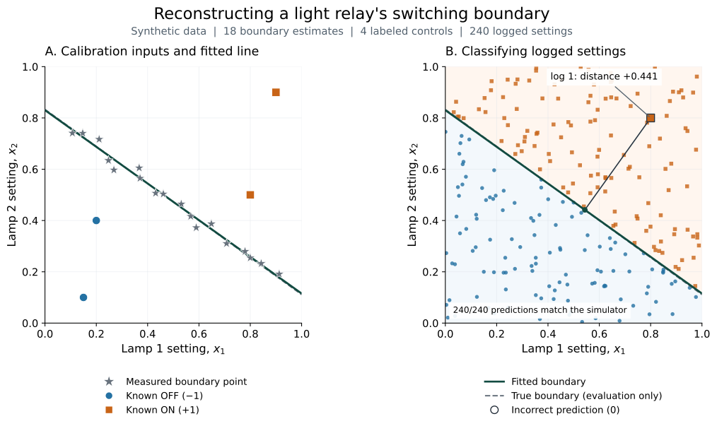
\[0.65x_1+0.90x_2-0.75>0\]and OFF otherwise. These coefficients are used to generate the data and evaluate the predictions; they are not supplied to the fitting function. The fixed random seed is 20171006. We generate 18 boundary measurements with independent Gaussian noise of standard deviation \(0.018\) in each recorded coordinate, four labeled controls, and 240 logged settings. The first three logged settings are chosen for illustration; the other 237 are sampled uniformly from the unit square. Their true labels are kept in a separate evaluation file.

The stars are noisy switching-point measurements. Blue circles represent OFF and orange squares represent ON: the left panel shows known labels, while the right panel shows predictions. The dashed line is the simulator’s true boundary, included only as an evaluation reference. It nearly overlaps the fitted line. A vector version of the figure is available for download.
Fitting the boundary points and choosing the orientation from the four labeled controls gives the following classifier, with coefficients rounded to six decimal places:
\[f(\vec x)=0.581682x_1+0.813416x_2-0.675409.\]The unrounded normal has unit length, so the score is the signed distance in the normalized feature coordinates. Positive scores predict ON; zero or negative scores predict OFF. The first three predictions are:
| Log ID | Lamp 1 | Lamp 2 | Signed distance | Predicted state |
|---|---|---|---|---|
| 0 | 0.15 | 0.20 | -0.425473 | OFF |
| 1 | 0.80 | 0.80 | +0.440670 | ON |
| 2 | 0.50 | 0.47 | -0.002262 | OFF |
Log 2 lies very close to the fitted boundary, so a small measurement change could alter its predicted state. Its distance is not a probability. With this seed, all 240 predictions match the simulator, and the root-mean-square distance of the boundary measurements to the fitted line is about \(0.0171\). This deliberately simple example demonstrates the workflow; it is not a benchmark of performance on real data.
A Runnable Python Example
The implementation is split into boundary_classifier.py, which fits and orients the hyperplane, and generate_example.py, which creates the synthetic data, evaluates predictions, and produces the figure. The fitting function accepts points in any dimension; the demonstration uses two dimensions so that its geometry can be plotted.
The core calculation below can be run from the example directory. It reads only boundary measurements, orientation labels, and unlabeled settings:
import numpy as np
from boundary_classifier import fit_hyperplane, orient_hyperplane

boundary = np.loadtxt("boundary_points.csv", delimiter=",", skiprows=1)
controls = np.loadtxt("orientation_points.csv", delimiter=",", skiprows=1)
logs = np.loadtxt("unlabeled_points.csv", delimiter=",", skiprows=1)

w, b = fit_hyperplane(boundary)
w, b = orient_hyperplane(w, b, controls[:, :2], controls[:, 2])

signed_distances = logs[:, 1:3] @ w + b  # The first column is the log ID.
predicted_labels = np.where(signed_distances > 0, 1, -1)
print(np.column_stack((logs[:3, 0], signed_distances[:3], predicted_labels[:3])))
fit_hyperplane centers the points and uses the last right singular vector as the unit normal. It checks for insufficient affine rank and a numerically non-unique smallest singular direction. orient_hyperplane compares the two possible orientations against the known labels and reports a tie instead of choosing a class assignment arbitrarily. The centered matrix has at least as many rows as columns, so its reduced SVD retains every right singular vector. This differs from applying a reduced SVD to the wide direction matrix in the exact construction earlier in the article.
Download and extract the complete example bundle. From its boundary-points directory, the following commands create an environment, run the classifier on the supplied CSV files, and regenerate the data and figure:
python3.12 -m venv .venv
. .venv/bin/activate
python -m pip install -r requirements.txt
python boundary_classifier.py
python generate_example.py
The example was run with Python 3.12.12. The generator resolves output paths relative to its own file, and accepts --output-dir to write a separate copy or --seed to try another sample. Regeneration overwrites its named output files. The supplied requirements.txt records the NumPy and Matplotlib versions used here, and the README documents the commands and file schemas.
All data and results are also available individually:
- boundary_points.csv: the 18 noisy boundary measurements used for fitting.
- orientation_points.csv: four labeled controls used to assign ON/OFF to the two sides.
- unlabeled_points.csv: the 240 logged settings to classify.
- evaluation_truth.csv: simulator labels and true distances, used only for evaluation.
- predictions.csv: predicted labels and signed distances, matched to the input logs by
log_id. - results.json: full-precision coefficients, the random seed, noise settings, diagnostics, and software versions.
References
- Active Decision Boundary Annotation with Deep Generative ModelsIn Proceedings of the IEEE International Conference on Computer Vision (ICCV), 2017
- Random Sample Consensus: A Paradigm for Model Fitting with Applications to Image Analysis and Automated CartographyCommunications of the ACM, 1981
Enjoy Reading This Article?
Here are some more articles you might like to read next:
- Google Gemini updates: Flash 1.5, Gemma 2 and Project Astra
- Displaying External Posts on Your al-folio Blog
- Binary Circles, Hamiltonian Cycles and de Bruijn Sequences
- Almost-Equal Isosceles Triangles: When Height Nearly Matches Base
- Building Intelligent Agents for Connect-4: Final Considerations
- Building Intelligent Agents for Connect-4: Verification and Benchmarking
- The Hexadecimal Digit Canon Challenge: Solution
- Building Intelligent Agents for Connect-4: MTD(f) and Null-Window Search
- Building Intelligent Agents for Connect-4: Opening Databases
- Building Intelligent Agents for Connect-4: Transposition Tables