Online Estimation: The Covariance of a Weighted Mean

• Paired Observations and Fixed Weights
• Expanding the Covariance
• Vector Form and Standard Errors
• The Covariance Correction is not a Mean Normalization
• Temporally Correlated Streams
• References

This post is the 5th part of a series of 7 articles:

1. Online Estimation: Learning from a Changing Data Stream
2. Online Estimation: The Mean and the Covariance Matrix
3. Online Estimation: Weighted Observations and Mini-Batches
4. Online Estimation: Exponential Forgetting
5. Online Estimation: The Covariance of a Weighted Mean
6. Online Estimation: The Memory of an Exponentially Weighted Estimator
7. Online Estimation: Updating the Inverse Covariance Matrix

An estimated covariance describes the spread of the observations, whereas the covariance of an estimated mean describes how that mean would vary across repeated datasets. These are different objects with different interpretations, they are very easy to conflate, and the second one is what we need in order to explain the memory of a forgetting estimator in the next article. For an ordinary unweighted mean the second quantity shrinks to zero as the sample grows, which is the usual reason for not thinking about it very hard. Under fixed exponential forgetting it does not, and that is the whole subject of the two articles which follow.

Appendix B.2.3 of my thesis (Thill, 2022) derives the result by expanding two weighted means and separating the terms with matching observation indices from those with different indices. I retain that route here and write it out in full, since the interesting work happens in the middle of the chain and the independence assumptions are what make the off-diagonal terms collapse.

Paired Observations and Fixed Weights

Let \((X_i,Y_i)\) be independent and identically distributed pairs of jointly distributed random variables, with common means \(\mu_X,\mu_Y\) and finite second moments. The two components within a pair may be correlated, which is the whole point of computing a covariance at all; independence is assumed only between different observation indices. The covariance of two jointly distributed random variables is

and the two weighted sample means whose covariance we want are

Taking the weights to be fixed, nonnegative and already normalized, \(w_i=w'_i/W_n\) with \(W_n=\sum_iw'_i\) and therefore \(\sum_iw_i=1\), these become \(\bar X_n=\sum_iw_iX_i\) and \(\bar Y_n=\sum_iw_iY_i\), so that

Since the weights are fixed and every observation has the same mean, \(\mathbb{E}[\bar X_n]=\sum_iw_i\mu_X=\mu_X\) and likewise \(\mathbb{E}[\bar Y_n]=\mu_Y\). It is worth keeping the normalization \(w_i=w'_i/W_n\) in view throughout, because the whole difficulty at the end of this article comes from substituting a different denominator by mistake.

Expanding the Covariance

Multiplying out the two sums and splitting the resulting double sum along its diagonal gives

The split is the substantive step. The first sum collects the paired, mutually dependent observations \((X_i,Y_i)\), which share one index and therefore cannot be decoupled; the appendix prints \(X_iY_j\) in this diagonal sum even though only \(i\) is bound by it, which is a typographical slip that does not affect the result but does obscure why the two sums have to be treated differently. All remaining pairs \(\{(X_i,Y_j)\mid i\ne j\}\) are statistically independent. Using linearity of expectation and then pulling the fixed weights out,

where the last line uses \(\mathbb{E}[XY]=\mathbb{E}[X]\mathbb{E}[Y]\) for independent \(X\) and \(Y\), which applies to the off-diagonal terms only. Since \(\mathbb{E}[X_i]=\mu_X\) and \(\mathbb{E}[Y_j]=\mu_Y\) for every index, the off-diagonal expectations are all the same constant and can be taken outside:

On the diagonal we cannot factor the expectation, but we can apply the definition of covariance in reverse, \(\mathbb{E}[X_iY_i]=\operatorname{Cov}(X_i,Y_i)+\mu_X\mu_Y\), and then separate the two contributions:

The diagonal and off-diagonal weight sums are exactly the two halves the original double sum was split into, so putting them back together and using \(\sum_jw_j=1\) twice makes the mean-product terms cancel:

Finally, since all pairs are identically distributed they share one covariance, and we are left with

Vector Form and Standard Errors

Applying the scalar calculation to every pair of coordinates of IID random vectors \(\mathbf{X}_i\) with covariance \(\boldsymbol{\Sigma}\) gives

and equal weights \(w_i=1/n\) recover the familiar \(\boldsymbol{\Sigma}/n\). For coordinate \(j\), the variance of the mean is \(\Sigma_{jj}\sum_iw_i^2\) and its standard error is the square root of that, so describing \(\sigma^2/n\) as a standard error, as is easily done in passing, confuses the two quantities.

No Gaussian assumption entered this derivation anywhere. If the observations happen to be Gaussian then a weighted mean is exactly Gaussian, being a linear combination of independent Gaussian vectors, and for general non-Gaussian data \eqref{eq:cov-weighted-mean} remains exact while normality requires a separate argument or approximation. That distinction matters more than it might appear for forgetting estimators: with fixed exponential forgetting, simply increasing the number of observations does not make the largest normalized weight vanish, so an ordinary central limit theorem cannot automatically justify an asymptotically exact normal approximation in that setting.

The Covariance Correction is not a Mean Normalization

The mean’s denominator is \(W_n\), whereas the reliability-weight covariance denominator derived two articles ago is \(W_n-W_n^{(2)}/W_n\). Substituting the latter into the mean’s weights breaks \(\sum_iw_i=1\) and therefore inflates the predicted covariance of the mean. It is a natural substitution to make, since both expressions are denominators built from the same two weight sums, and unlike a sign error it produces entirely plausible numbers rather than an obvious failure.

import numpy as np

lam, n, population_variance = .99, 500, 3.
raw = lam**np.arange(n-1, -1, -1)
W, Q = raw.sum(), raw @ raw
weights = raw/W
assert np.isclose(weights.sum(), 1.)
variance_of_mean = population_variance * (weights @ weights)
standard_error = np.sqrt(variance_of_mean)
print(variance_of_mean)  # about 0.0152747922
print(standard_error)    # about 0.1235912301

Using the covariance denominator in this example predicts about \(0.015431534\) instead of \(0.015274792\), an overstatement of roughly one percent, and stronger forgetting makes the error considerably more visible. The assertion on the normalized weights is the cheapest possible guard against the whole class of mistake.

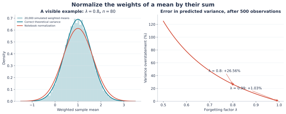
The plot generator and the companion notebook contain the reproducible calculations, and the notebook displays the theoretical standard deviations explicitly rather than drawing a curve from an empirical value and calling it theory.

Temporally Correlated Streams

Without independence across indices, the off-diagonal expectations no longer factor and the general expression is

in which the cross-index terms need not disappear. Consequently the same weight schedule can produce quite different uncertainty on an autocorrelated stream, which is a real limitation given that the motivating application in my thesis was time series anomaly detection. Random or data-dependent weights require additional care for the same reason, since they cannot simply be treated as fixed coefficients independent of the observations.

Under the IID assumptions, though, we have a particularly simple answer: uncertainty in the mean depends only on the sum of squared normalized weights. Taking the reciprocal of that sum gives the effective memory derived in the next article.

Source: thesis Appendix B.2.3, covSampleMeans through covSampleMeansNormalized5. The diagonal sum is written with matching indices \(X_iY_i\), and the variance of the mean is distinguished from its standard error.

References