Online Estimation: Exponential Forgetting

• Exponential Weights at Batch Boundaries
• The Mean Update
• The Scatter Update and its Historical Means
• The Fully Online Case
• What Changes when we Batch Observations
• References

This post is the 4th part of a series of 7 articles:

1. Online Estimation: Learning from a Changing Data Stream
2. Online Estimation: The Mean and the Covariance Matrix
3. Online Estimation: Weighted Observations and Mini-Batches
4. Online Estimation: Exponential Forgetting
5. Online Estimation: The Covariance of a Weighted Mean
6. Online Estimation: The Memory of an Exponentially Weighted Estimator
7. Online Estimation: Updating the Inverse Covariance Matrix

The weighted update of the previous article becomes considerably more useful once old observations are allowed to gradually lose influence. Appendix B.2.2 of my thesis (Thill, 2022) chooses exponentially decaying weights for this, and the reason is worth stating plainly: it is the one weighting scheme in which all historical weights can change at every step without our ever having to revisit the historical data. Any other schedule either keeps the old observations around or quietly approximates something.

We will derive the update in the same step-by-step way as before, then look carefully at what a forgetting factor actually means for a mini-batch. Along the way two corrections to the appendix are needed. One is a missing superscript in the summary equation for the squared-weight sum, which changes a covariance denominator; the other concerns the means which appear when the scatter recurrence is unrolled, and a three-point counterexample settles it in exact arithmetic. Neither affects the final algorithm, which is correct as printed.

Exponential Weights at Batch Boundaries

Let every batch contain \(\mu\) observations, and suppose \(n=M\mu\) observations have arrived in \(M\) batches, so that observation \(i\) belongs to batch \(j=\lceil i/\mu\rceil\). At this boundary, assign it the weight

All \(\mu\) observations in the most recent batch then carry \(w'_k=\cdots=w'_n=1\), the penultimate batch carries \(w'_{n-2\mu+1}=\cdots=w'_{n-\mu}=\lambda\), and so on backwards, so that for \(\lambda<1\) the older batches fade away exponentially. Two practical advantages follow: the weight sum and the scatter matrix stay bounded instead of growing without limit, and the estimates can adapt to new conditions in a non-stationary environment.

For \(\lambda<1\) the geometric sum gives the normalization factor in closed form,

These closed forms are valid only for \(\lambda<1\); the case \(\lambda=1\) has to be read off directly, and gives \(W_n=W_n^{(2)}=n\).

When a new batch arrives, every weight \(\{w'_i\mid i\le n-\mu\}\) is multiplied by \(\lambda\) and the incoming observations are given weight one. Ordinarily, changing every weight would force a recomputation of both statistics from scratch. The point of this particular schedule is that it does not, and the next three sections show why. Starting from

we can split the newest batch off the sum defining \(W_n\) and recognize what remains:

The same argument applied to squared weights gives

where the decay factor is squared because the weights themselves are. The corresponding summary equation in the appendix propagates \(W_{n-1}\) rather than \(W_{n-1}^{(2)}\) on the right-hand side, and that missing superscript has real consequences: for \(\lambda=1/2\) and three observations the correct squared-weight sum is \(21/16\), while the printed version gives \(11/8\). Since \(W_n^{(2)}\) enters the denominator \(W_n-W_n^{(2)}/W_n\) of the unbiased weighted covariance, the difference propagates straight into the reported estimate. The general batch form elsewhere in the appendix is correct, so this is an erratum in the specialization rather than in the derivation. Both recurrences remain valid at \(\lambda=1\), where they reproduce \(W_n=W_n^{(2)}=n\).

The Mean Update

It is convenient to write \(\boldsymbol{\sigma}_j\) for the plain sum of the observations in batch \(j\), so that with \(n_j=j\mu\) and \(k_j=n_j-\mu+1=\mu(j-1)+1\),

because every observation within a batch carries the same weight \(\lambda^{M-j}\). The previous mean and the previous normalization factor are

the second of which is just the weight recurrence rearranged. Splitting the newest batch off the numerator and substituting both then gives the increment:

with \(k=n-\mu+1\) and \(\boldsymbol{\Delta}_i=\mathbf{x}_i-\bar{\mathbf{x}}_{n-\mu}\) as in the previous article. The sixth line uses \(\mu\bar{\mathbf{x}}_{n-\mu} =\sum_{i=k}^n\bar{\mathbf{x}}_{n-\mu}\), which is only a way of writing one term as a sum over the batch so that the two sums can be combined. Note that this is the same increment as in the general weighted case, with all incoming weights equal to one; the decay has been absorbed entirely into \(W_n\).

The Scatter Update and its Historical Means

There is a short argument which avoids repeating the algebra of the previous article. Multiplying all old weights by \(\lambda\) leaves their weighted mean unchanged, since the factor cancels between numerator and denominator, and multiplies their scatter by \(\lambda\), since the scatter is linear in the weights. We may therefore apply the weighted batch update to this rescaled old state, assigning unit weights to the incoming observations, which gives

The appendix instead reaches the same recurrence by unrolling the general batch update, which is worth reproducing because it is the more instructive route, provided one point is fixed. Write \(\boldsymbol{\Delta}^{(j)}_i=\mathbf{x}_i-\bar{\mathbf{x}}_{n_j-\mu}\) for the residual of observation \(i\) against the mean which was current when batch \(j\) arrived. Unrolling the weighted batch update of the previous article from an empty state then gives

where the last line identifies

The point to fix is that each historical increment must keep the two means which were current when it was formed, namely \(\bar{\mathbf{x}}_{n_j-\mu}\) inside \(\boldsymbol{\Delta}^{(j)}_i\) and \(\bar{\mathbf{x}}_{n_j}\) in the right-hand factor. The appendix writes the current \(\bar{\mathbf{x}}_n\) in every historical term, and with that reading the identification in the last line does not hold, because the displayed sum is then not \(\bar{\mathbf{M}}^{(n-\mu)}\). A three-point counterexample settles it in exact arithmetic: with \(x_1=0\), \(x_2=2\), \(x_3=4\), \(\mu=1\), \(\lambda=1/2\) and zero initial state, the means are \(0\), \(4/3\) and \(20/7\); the direct weighted scatter and the recurrence \eqref{eq:forgetting-scatter} both give \(26/7\), while the printed historical sum gives \(46/21\).

The direct definition of the weighted scatter, which centers every observation about the latest mean, remains perfectly valid of course. It is simply a different expansion from this sum of historical increments, and the two must not be mixed.

The Fully Online Case

For \(\mu=1\) the whole algorithm is five lines, processed in this order:

The second line is \eqref{eq:squared-weight-recurrence} at \(\mu=1\), with the previous sum of squared weights on the right; this is the equation whose superscript is missing in the appendix. Divide the scatter by \(W_n\) for the population normalization, or by \(W_n-W_n^{(2)}/W_n\) for the reliability-weight correction. Under genuine drift the IID assumptions behind the word “unbiased” need not hold at all, even though the weighted arithmetic itself remains exact.

For large \(n\) and fixed \(\lambda<1\) the factor \(1/W_n\) approaches \(1-\lambda\), which is the form usually quoted, but keeping the finite weight sum handles the startup phase explicitly and costs one scalar. There is also no need to perturb \(\lambda=1\) to a nearby number in an implementation: it represents the valid no-forgetting case, and the recurrences above are well defined there even though the geometric closed forms are not.

What Changes when we Batch Observations

If an online estimator and a batch estimator are both configured with decay=0.98, the batch estimator forgets only once per batch, so for batches of 20 observations it retains very much more history measured in observations. This follows directly from \eqref{eq:exp-weights}, in which the exponent counts batches rather than observations, and it is the sort of difference which shows up as a puzzling discrepancy between two implementations that were supposed to agree.

To reproduce per-observation forgetting with factor \(r\) using a batch, consider a new batch of size \(b\). At its end, all old weights must have been multiplied by \(r^b\), and within the new batch the first observation must have weight \(r^{b-1}\) while the last has weight one. Both changes are required for exact agreement; setting only decay=r**b and retaining equal weights within each batch gives a useful but different weighting scheme.

import numpy as np
from online_estimation import IncrementalMoments

rng = np.random.default_rng(20260315)
X = rng.normal(size=(60, 2))
r = .98
online = IncrementalMoments(2, decay=r)
batched = IncrementalMoments(2)
for batch in np.array_split(X, 6):
    for row in batch:
        online.update(row)
    b = len(batch)
    batched.update(batch, decay=r**b,
                   weights=r**np.arange(b-1, -1, -1))
    np.testing.assert_allclose(batched.mean, online.mean, atol=1e-12)
    np.testing.assert_allclose(batched.covariance(), online.covariance(), atol=1e-12)

Use online_estimation.py for this example.

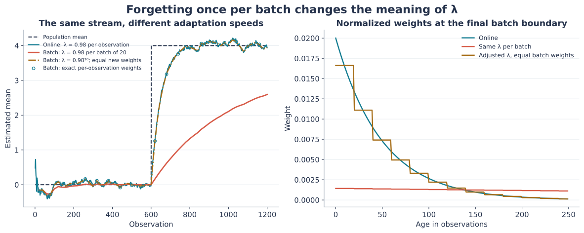
The companion notebook verifies mean and covariance agreement at every batch boundary, across decay factors 1, 0.5 and 0.99 and across unequal incoming weights. The next two articles quantify the remaining noise in the mean and explain how to translate a forgetting factor into a variance-equivalent sample size.

Source: thesis Appendix B.2.2, including weighted-mean-batch and final-exp-decay-scatter. The historical means in the unrolled expansion and the missing superscript in the squared-weight summary are corrected as documented in the derivation review.

References