Online Estimation: Updating the Inverse Covariance Matrix

• From Scatter to Covariance and Precision
• The Batch Update in Matrix Form
• Applying the Woodbury Identity
• The Single-Observation Specialization
• The Update Rules in Summary
• An Inverse cannot be Initialized Independently
• Verifying the Covariance that is Actually Reported
• Cost and Numerical Limits
• References

This post is the 7th part of a series of 7 articles:

1. Online Estimation: Learning from a Changing Data Stream
2. Online Estimation: The Mean and the Covariance Matrix
3. Online Estimation: Weighted Observations and Mini-Batches
4. Online Estimation: Exponential Forgetting
5. Online Estimation: The Covariance of a Weighted Mean
6. Online Estimation: The Memory of an Exponentially Weighted Estimator
7. Online Estimation: Updating the Inverse Covariance Matrix

In practice one often needs the inverse of a covariance matrix rather than the covariance itself, the Mahalanobis distance being the obvious example. In a fully online setting, recomputing that inverse for every arriving observation is expensive, since inverting a \(d\times d\) matrix costs about \(O(d^3)\), only slightly less in the more elaborate algorithms. Appendix B.2.2.1 of my thesis (Thill, 2022) shows that this is avoidable in two senses: the covariance itself need never be formed if only its inverse is wanted, and the inverse can be updated incrementally. The tools are the Woodbury identity (Woodbury, 1950) for batches and its Sherman-Morrison specialization (Sherman & Morrison, 1950) for a single observation, and the results below are stated for the general weighted, exponentially decaying estimator.

Both identities require an existing inverse to update, which means that handling the first observations is part of the algorithm rather than an implementation detail to be papered over. That turns out to be where the practical difficulty lies, and this article spends as much space on initialization as on the identities themselves.

From Scatter to Covariance and Precision

We now write \(\bar{\mathbf{M}}_n\) in place of \(\bar{\mathbf{M}}^{(n)}\), moving the superscript to the index as the thesis does at this point, so that inverses can be written without ambiguity. If the covariance estimate is \(\bar{\boldsymbol{\Sigma}}_n=\bar{\mathbf{M}}_n/c_n\) for a positive scalar \(c_n\), then

where \(c_n=W_n\) gives the population normalization and \(c_n=W_n-W_n^{(2)}/W_n\) the reliability-weight correction. Note that scaling the inverse requires multiplication by \(c_n\) rather than division, which is easy to get backwards when switching between the two normalizations. It is also worth stating that the inverse of an unbiased covariance estimate is not generally an unbiased estimate of the population precision; unbiasedness does not survive matrix inversion, and nothing in this article claims that it does.

The Batch Update in Matrix Form

The scatter recurrence from the fourth article is a sum of \(\mu\) outer products, and writing it as a single matrix product is what exposes its low-rank structure. For an incoming batch of size \(\mu\), define the two \(\mu\times d\) matrices

where \(k=n-\mu+1\) and \(\boldsymbol{\Delta}_i=\mathbf{x}_i-\bar{\mathbf{x}}_{n-\mu}\) as before. The first collects the residuals against the old mean as its rows and the second those against the new mean, so that

in which the product \(\mathbf{D}_n^T\boldsymbol{\mathcal{X}}_n\) has size \(d\times d\), as required, while its inner dimension is only \(\mu\). The identity matrix is written explicitly because it is what plays the role of \(\mathbf{C}\) below. For arbitrary incoming weights, replace \(\boldsymbol{\mathcal{X}}_n\) by \(\operatorname{diag}(w'_k,\ldots,w'_n)\boldsymbol{\mathcal{X}}_n\).

Applying the Woodbury Identity

For compatible matrices possessing the needed inverses, the Woodbury identity reads

The expression inside the inner inverse contains the product \(\mathbf{V}\mathbf{A}^{-1}\mathbf{U}\). The thesis prints a plus sign where the second multiplication belongs, giving \(\mathbf{C}^{-1}+\mathbf{V}\mathbf{A}^{-1}+\mathbf{U}\), which is not even dimensionally defined for the rectangular batch matrices above, since \(\mathbf{V}\mathbf{A}^{-1}\) is \(\mu\times d\) while \(\mathbf{U}\) is \(d\times\mu\). The specialized batch update which the thesis then derives already carries the correct product, so this is a typographical slip in the statement of the general identity rather than an error in the result. With

substitution into \eqref{eq:woodbury} gives, using \(\mathbf{A}^{-1}=\lambda^{-1}\bar{\mathbf{M}}_{n-\mu}^{-1}\) in three places,

The step between the two lines pulls a factor \(\lambda\) out of the inner inverse: writing \(\mathbf{B}=\boldsymbol{\mathcal{X}}_n\bar{\mathbf{M}}_{n-\mu}^{-1}\mathbf{D}_n^T\), we have \(\big(\mathbf{I}+\lambda^{-1}\mathbf{B}\big)^{-1} =\big(\lambda^{-1}(\lambda\mathbf{I}+\mathbf{B})\big)^{-1} =\lambda\big(\lambda\mathbf{I}+\mathbf{B}\big)^{-1}\), and that factor cancels one of the two powers of \(\lambda\) in front. Writing \(\mathbf{P}_{\mathrm{old}}=\bar{\mathbf{M}}_{n-\mu}^{-1}\) and collecting, the update is

The inner system has dimension \(\mu\) rather than \(d\), which is the entire point of the exercise, and in code one should solve that system rather than explicitly forming its inverse. Since an inverse still has to be computed somewhere, the identity is only worth using when the batch size \(\mu\) is appreciably smaller than the dimension \(d\) of the observations.

The Single-Observation Specialization

For \(\mu=1\) the inner system is scalar, and the Woodbury identity reduces to the Sherman-Morrison formula,

Reading the fully online scatter recurrence \(\bar{\mathbf{M}}_n=\lambda\bar{\mathbf{M}}_{n-1}+\boldsymbol{\Delta}_n(\mathbf{x}_n-\bar{\mathbf{x}}_n)^T\) as \(\mathbf{A}+\mathbf{u}\mathbf{v}^T\), we identify

and substituting \(\mathbf{A}^{-1}=\lambda^{-1}\bar{\mathbf{M}}_{n-1}^{-1}\) gives a numerator carrying \(\lambda^{-2}\) and a denominator \(1+\lambda^{-1}\mathbf{v}^T\bar{\mathbf{M}}_{n-1}^{-1}\mathbf{u} =\lambda^{-1}\big(\lambda+\mathbf{v}^T\bar{\mathbf{M}}_{n-1}^{-1}\mathbf{u}\big)\). One power of \(\lambda\) cancels between them, leaving

The two matrix-vector products should be computed first and only then combined into an outer product. This is worth saying because a left-associated sequence of matrix multiplications, which is what one gets by transcribing the formula naively, quietly introduces a dense matrix-matrix multiplication into what should be an \(O(d^2)\) update, and the resulting implementation can be slower than simply calling a solver.

The Update Rules in Summary

Processed in this order, a batch running from \(k=n-\mu+1\) to \(n\) gives

and for the fully online case \(\mu=1\), \(k=n\), these simplify to

Both summaries use the population normalization in the last line; for an unbiased covariance use the reliability-weight denominator \(W_n-W_n^{(2)}/W_n\) instead, and remember to multiply rather than divide when converting the inverse. Both squared-weight recurrences carry the previous sum of squared weights on their right-hand side, which is the missing superscript noted in the fourth article.

An Inverse cannot be Initialized Independently

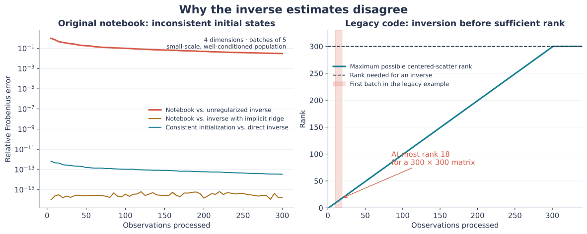
A centered sample scatter has rank at most \(\min(d,n-1)\), so in 300 dimensions a first batch of 10 to 19 observations is necessarily singular, and no choice of solver repairs it. Since the identities above update an existing inverse rather than producing one, the first few observations need an explicit decision.

Setting the scatter to zero while setting its inverse to \(c\mathbf{I}\) is not such a decision, because those two matrices are not a matrix and its inverse in any sense: their product is zero rather than the identity. Subsequent Woodbury updates then track the inverse of a scatter carrying an implicit initial ridge \(c^{-1}\mathbf{I}\), whose remaining contribution after \(t\) forgetting updates is \(\lambda^tc^{-1}\mathbf{I}\). The difficulty is not the ridge itself, which is a perfectly reasonable thing to want, but that the reported covariance does not include it, so the maintained inverse and the reported covariance describe two different matrices.

There are two defensible choices, and the important thing is to make one of them explicitly:

• Warm up from zero scatter. Accumulate observations until the scatter is positive definite and sufficiently well conditioned, initialize its inverse by a direct solve, and only then update it incrementally.
• Use a declared regularized scatter. Initialize \(\bar{\mathbf{M}}_0=\rho\mathbf{I}\) together with \(\bar{\mathbf{M}}_0^{-1}=\rho^{-1}\mathbf{I}\), state whether that ridge decays, and report the covariance corresponding to the regularized scatter rather than to an unregularized one.

The Python implementation uses warm-up, initializing the inverse only after a Cholesky check and a declared condition limit of \(10^{10}\). The adapted R example illustrates the second choice with \(\rho=0.01\) and hence an initial inverse of \(100\mathbf{I}\); initializing both matrices to \(0.01\mathbf{I}\), which is the natural-looking but inconsistent choice, gives a product of \(10^{-4}\mathbf{I}\). Forgetting does hide such a discrepancy after a long run, but the early estimates then do not describe the same matrix, so the script compares the maintained inverse against the inverse of the same regularized scatter throughout rather than only at the end. Its regularized covariance is not labeled an unbiased sample covariance.

Verifying the Covariance that is Actually Reported

Run the following beside online_estimation.py:

import numpy as np
from online_estimation import IncrementalMoments

rng = np.random.default_rng(20260426)
X = .01*rng.normal(size=(40, 4))
state = IncrementalMoments(4, track_inverse=True)
state.update(X[:4])
assert state.scatter_inverse is None
for batch in np.array_split(X[4:], 6):
    state.update(batch)
reference_cov = np.cov(X, rowvar=False)
reference_precision = np.linalg.solve(reference_cov, np.eye(4))
np.testing.assert_allclose(state.covariance(), reference_cov, atol=1e-12)
np.testing.assert_allclose(state.precision(), reference_precision, rtol=1e-9)
np.testing.assert_allclose(state.covariance() @ state.precision(), np.eye(4), atol=1e-9)

With forgetting enabled, the reference must be an explicitly weighted one rather than np.cov(X) without weights, which otherwise produces a comparison that can only fail for reasons unrelated to the update. The companion notebook checks variable batches and scales, inverse residuals, symmetry, startup, and the no-forgetting limit, across 450 inverse comparisons whose maximum relative error is about \(1.97\cdot10^{-13}\) and whose maximum covariance-times-precision residual is about \(1.50\cdot10^{-12}\).

Cost and Numerical Limits

A batch update still requires matrix products in addition to the smaller solve, at an approximate cost of \(O(d^2\mu+d\mu^2+\mu^3)\), so whether it is actually faster depends on the dimensions, the implementation and the hardware. A small batch can certainly help, but \(\mu<d\) on its own guarantees nothing, and the timings in the notebook are machine-specific for exactly this reason.

The identities are exact algebraically, while repeated inverse updates accumulate floating-point error, and the two statements are not in conflict. In a long-running system it is worth monitoring conditioning and residuals and refactoring the inverse when necessary. Symmetrizing a result can remove small roundoff asymmetries but cannot repair a genuinely singular estimate, and when only a few Mahalanobis scores are needed, applying a Cholesky solve may well be preferable to storing a full inverse at all.

This completes the path from ordinary sample statistics through weighted batches, forgetting, uncertainty of the mean and finally inverse updates. Each stage uses the same mean-and-scatter state, with the statistical interpretation and the startup conditions kept explicit throughout.

Source: thesis Appendix B.2.2.1. The general Woodbury identity is stated with the product \(\mathbf{V}\mathbf{A}^{-1}\mathbf{U}\) inside the inner inverse, and the inverse initialization is made consistent with the scatter it is supposed to invert.

References

- Machine Learning and Deep Learning Approaches for Multivariate Time Series Prediction and Anomaly DetectionLeiden University, 2022
- Inverting Modified Matrices1950
- Adjustment of an Inverse Matrix Corresponding to a Change in One Element of a Given MatrixThe Annals of Mathematical Statistics, 1950
Enjoy Reading This Article?
Here are some more articles you might like to read next:
- Google Gemini updates: Flash 1.5, Gemma 2 and Project Astra
- Displaying External Posts on Your al-folio Blog
- Constructing a Linear Classifier from Known Decision-Boundary Points
- Binary Circles, Hamiltonian Cycles and de Bruijn Sequences
- Almost-Equal Isosceles Triangles: When Height Nearly Matches Base
- Building Intelligent Agents for Connect-4: Final Considerations