Online Estimation: The Mean and the Covariance Matrix
This post is the 2nd part of a series of 7 articles:
- Online Estimation: Learning from a Changing Data Stream
- Online Estimation: The Mean and the Covariance Matrix
- Online Estimation: Weighted Observations and Mini-Batches
- Online Estimation: Exponential Forgetting
- Online Estimation: The Covariance of a Weighted Mean
- Online Estimation: The Memory of an Exponentially Weighted Estimator
- Online Estimation: Updating the Inverse Covariance Matrix
The ordinary mean and covariance provide a useful starting point for online estimation. Their definitions involve all observations, and yet their updates need only the previous state and the newest vector, which is the pattern every later article in this series will follow. Appendix B.2.1 of my thesis (Thill, 2022) arrives at this by updating an unnormalized scatter matrix first and choosing a covariance normalization afterwards, and since that separation turns out to be exactly what the weighted and forgetting cases need as well, I will keep it here.
This article treats the unweighted case with one observation at a time, which is the specialization of the thesis derivation to unit weights and batch size one. Doing it separately first is worth the duplication, because the general derivation in the next article has the same shape but carries weight sums through every line, and it is easier to follow once the plain version is familiar. The derivation is elementary throughout, but it has one step which is easy to state carelessly: the two residuals in the scatter update are taken with respect to two different means, and that asymmetry is not a typographical accident.
Definitions and the Two Covariance Normalizations
For observations \(\mathbf{x}_1,\ldots,\mathbf{x}_n\in\mathbb{R}^d\), define
\[\bar{\mathbf{x}}_n=\frac{1}{n}\sum_{i=1}^n\mathbf{x}_i,\qquad \bar{\mathbf{M}}^{(n)}=\sum_{i=1}^n (\mathbf{x}_i-\bar{\mathbf{x}}_n)(\mathbf{x}_i-\bar{\mathbf{x}}_n)^T.\]For IID observations with finite covariance, the usual unbiased covariance estimate is \(\bar{\mathbf{M}}^{(n)}/(n-1)\), whereas for a Gaussian model whose mean is estimated from the same observations, the covariance maximum-likelihood estimate is \(\bar{\mathbf{M}}^{(n)}/n\). These are two different normalizations of one and the same scatter matrix, and the distinction is worth keeping straight, since the two names are often used interchangeably even though only one of them is unbiased. This is also the reason for storing the scatter itself as the state and deciding on the denominator only when a covariance is actually reported. In the convergence examples below we use the unbiased version throughout.
Updating the Mean
Separating the newest observation from the sum and then adding and subtracting the old mean gives the update in four short steps:
\[\begin{aligned} \bar{\mathbf{x}}_n &=\frac{1}{n}\sum_{i=1}^n\mathbf{x}_i\\ &=\frac{\sum_{i=1}^{n-1}\mathbf{x}_i+\mathbf{x}_n}{n} =\frac{(n-1)\bar{\mathbf{x}}_{n-1}+\mathbf{x}_n}{n}\\ &=\frac{n\bar{\mathbf{x}}_{n-1}-\bar{\mathbf{x}}_{n-1}+\mathbf{x}_n}{n}\\ &=\bar{\mathbf{x}}_{n-1}+\frac{\mathbf{x}_n-\bar{\mathbf{x}}_{n-1}}{n}. \end{aligned}\]If we define the residual
\[\begin{equation} \boldsymbol{\Delta}_n=\mathbf{x}_n-\bar{\mathbf{x}}_{n-1} \label{eq:delta-online} \end{equation}\]with respect to the previous mean, the update is simply \(\bar{\mathbf{x}}_n=\bar{\mathbf{x}}_{n-1}+\boldsymbol{\Delta}_n/n\), which costs \(O(d)\) arithmetic and needs no history beyond the running count. The second line above, \(n\bar{\mathbf{x}}_n=(n-1)\bar{\mathbf{x}}_{n-1}+\mathbf{x}_n\), is worth keeping in view, because the scatter derivation uses it twice.
Expanding the Scatter Matrix
It is convenient to first rewrite the scatter without any reference to the previous state. Expanding the outer product and keeping both cross terms until the summation is carried out gives
\[\begin{aligned} \bar{\mathbf{M}}^{(n)} &=\sum_{i=1}^n(\mathbf{x}_i-\bar{\mathbf{x}}_n)(\mathbf{x}_i-\bar{\mathbf{x}}_n)^T\\ &=\sum_{i=1}^n\left[\mathbf{x}_i\mathbf{x}_i^T -\mathbf{x}_i\bar{\mathbf{x}}_n^T -\bar{\mathbf{x}}_n\mathbf{x}_i^T +\bar{\mathbf{x}}_n\bar{\mathbf{x}}_n^T\right]\\ &=\sum_{i=1}^n\mathbf{x}_i\mathbf{x}_i^T -\left(\sum_{i=1}^n\mathbf{x}_i\right)\bar{\mathbf{x}}_n^T -\bar{\mathbf{x}}_n\left(\sum_{i=1}^n\mathbf{x}_i\right)^T +\sum_{i=1}^n\bar{\mathbf{x}}_n\bar{\mathbf{x}}_n^T\\ &=\sum_{i=1}^n\mathbf{x}_i\mathbf{x}_i^T -n\bar{\mathbf{x}}_n\bar{\mathbf{x}}_n^T -n\bar{\mathbf{x}}_n\bar{\mathbf{x}}_n^T +n\bar{\mathbf{x}}_n\bar{\mathbf{x}}_n^T\\ &=\sum_{i=1}^n\mathbf{x}_i\mathbf{x}_i^T-n\bar{\mathbf{x}}_n\bar{\mathbf{x}}_n^T. \end{aligned}\]The thesis compresses the two cross terms into a single \(-2\mathbf{x}_i\bar{\mathbf{x}}_n^T\) at the second line. That shortcut is harmless once the sum has been taken, since both sums do equal \(n\bar{\mathbf{x}}_n\bar{\mathbf{x}}_n^T\), but the individual matrix summands \(\mathbf{x}_i\bar{\mathbf{x}}_n^T\) and \(\bar{\mathbf{x}}_n\mathbf{x}_i^T\) are transposes of one another rather than equal, and writing them as a factor of two before summing invites the reader to believe otherwise. In the scalar case the distinction does not arise at all, which is precisely why it survives so easily when a scalar derivation is carried over to vectors.
Deriving the Scatter Update
Subtracting the corresponding expression at \(n-1\) removes all but the newest terms:
\[\begin{aligned} \bar{\mathbf{M}}^{(n)}-\bar{\mathbf{M}}^{(n-1)} &=\sum_{i=1}^n\mathbf{x}_i\mathbf{x}_i^T-n\bar{\mathbf{x}}_n\bar{\mathbf{x}}_n^T -\sum_{i=1}^{n-1}\mathbf{x}_i\mathbf{x}_i^T +(n-1)\bar{\mathbf{x}}_{n-1}\bar{\mathbf{x}}_{n-1}^T\\ &=\mathbf{x}_n\mathbf{x}_n^T-n\bar{\mathbf{x}}_n\bar{\mathbf{x}}_n^T +(n-1)\bar{\mathbf{x}}_{n-1}\bar{\mathbf{x}}_{n-1}^T. \end{aligned}\]The two mean identities from the previous section now do the work. We substitute \(n\bar{\mathbf{x}}_n=(n-1)\bar{\mathbf{x}}_{n-1}+\mathbf{x}_n\) into the second term, and its rearrangement \((n-1)\bar{\mathbf{x}}_{n-1}=n\bar{\mathbf{x}}_n-\mathbf{x}_n\) into the third, taking care to leave one factor \(\bar{\mathbf{x}}_{n-1}\) standing in the third term so that the substitution applies to the other:
\[\begin{aligned} \bar{\mathbf{M}}^{(n)}-\bar{\mathbf{M}}^{(n-1)} &=\mathbf{x}_n\mathbf{x}_n^T -\big[(n-1)\bar{\mathbf{x}}_{n-1}+\mathbf{x}_n\big]\bar{\mathbf{x}}_n^T +\bar{\mathbf{x}}_{n-1}\big[n\bar{\mathbf{x}}_n-\mathbf{x}_n\big]^T\\ &=\mathbf{x}_n\mathbf{x}_n^T -(n-1)\bar{\mathbf{x}}_{n-1}\bar{\mathbf{x}}_n^T -\mathbf{x}_n\bar{\mathbf{x}}_n^T +n\bar{\mathbf{x}}_{n-1}\bar{\mathbf{x}}_n^T -\bar{\mathbf{x}}_{n-1}\mathbf{x}_n^T\\ &=\mathbf{x}_n\mathbf{x}_n^T -\mathbf{x}_n\bar{\mathbf{x}}_n^T +\big[n-(n-1)\big]\bar{\mathbf{x}}_{n-1}\bar{\mathbf{x}}_n^T -\bar{\mathbf{x}}_{n-1}\mathbf{x}_n^T\\ &=\mathbf{x}_n\mathbf{x}_n^T -\mathbf{x}_n\bar{\mathbf{x}}_n^T +\bar{\mathbf{x}}_{n-1}\bar{\mathbf{x}}_n^T -\bar{\mathbf{x}}_{n-1}\mathbf{x}_n^T. \end{aligned}\]The four remaining terms group into two pairs sharing the right factor \((\mathbf{x}_n-\bar{\mathbf{x}}_n)^T\):
\[\begin{aligned} \bar{\mathbf{M}}^{(n)}-\bar{\mathbf{M}}^{(n-1)} &=\mathbf{x}_n\big(\mathbf{x}_n^T-\bar{\mathbf{x}}_n^T\big) -\bar{\mathbf{x}}_{n-1}\big(\mathbf{x}_n^T-\bar{\mathbf{x}}_n^T\big)\\ &=\big(\mathbf{x}_n-\bar{\mathbf{x}}_{n-1}\big) \big(\mathbf{x}_n-\bar{\mathbf{x}}_n\big)^T, \end{aligned}\]so that with \(\eqref{eq:delta-online}\) the online update is
\[\begin{equation} \bar{\mathbf{M}}^{(n)}=\bar{\mathbf{M}}^{(n-1)}+ \boldsymbol{\Delta}_n(\mathbf{x}_n-\bar{\mathbf{x}}_n)^T. \label{eq:scatter-online} \end{equation}\]The order of operations is the part worth remembering. We compute \(\boldsymbol{\Delta}_n\) using the old mean, then update the mean, and only then form the second residual against the new mean. Since \(\mathbf{x}_n-\bar{\mathbf{x}}_n=\mathbf{x}_n-\bar{\mathbf{x}}_{n-1}-\boldsymbol{\Delta}_n/n =(n-1)\boldsymbol{\Delta}_n/n\), the increment can equivalently be written as \((n-1)\boldsymbol{\Delta}_n\boldsymbol{\Delta}_n^T/n\), which makes it visibly symmetric and positive semidefinite. In practice the first form is the one to implement, because it is the form which generalizes to weights and mini-batches without modification.
In one dimension the same calculation reads
\[M_n=M_{n-1}+(x_n-\bar{x}_{n-1})(x_n-\bar{x}_n),\qquad s_n^2=\frac{M_n}{n-1},\]which is the familiar Welford-style recurrence. Note that although we used the raw second-moment expression to derive the identity, there is no reason to implement it that way: subtracting two potentially large and nearly equal matrices is precisely the catastrophic cancellation which \(\eqref{eq:scatter-online}\) avoids.
Initialization and a Small Example
Initialize the count and the scatter to zero. The first observation then sets the mean and leaves the scatter at zero, so the unbiased covariance is available only from the second observation onward, and a full matrix inverse generally needs considerably more than that. The last article of the series returns to this point, since for the inverse it is not merely a cosmetic detail.
For the scalar stream \(0,2,4,6\), the successive means are \(0,1,2,3\) and the scatters are \(0,2,8,20\), so that the final unbiased variance is \(20/3\). Processing the first two and last two values as batches has to give the same answer, and checking exactly that is a cheap way to catch an incorrect batch formula. The next article derives the required batch recurrence and returns to this example.
A compact R implementation of the central loop is:
# X: observations in rows. See the downloadable script for a full example.
running_mean <- rep(0, ncol(X))
scatter <- matrix(0, ncol(X), ncol(X))
for (n in seq_len(nrow(X))) {
  delta <- X[n, ] - running_mean
  running_mean <- running_mean + delta / n
  scatter <- scatter + tcrossprod(delta, X[n, ] - running_mean)
}
covariance <- if (nrow(X) > 1) scatter / (nrow(X) - 1) else NULL
The complete R script uses MASS::mvrnorm for the Gaussian sampling, together with a recorded seed, and defines the startup behavior explicitly rather than leaving the covariance undefined for a single observation.
A Reproducible Python Example
Place online_estimation.py beside the script below, or simply run it from the example directory. The implementation stores observations as rows, in the way NumPy users will expect, while the mathematical vectors in the derivation above remain column vectors.
import numpy as np
from online_estimation import IncrementalMoments

rng = np.random.default_rng(20260215)
mean = np.array([1., 10., 20.])
cov = np.array([[1., -1., .5], [-1., 3., -1.], [.5, -1., 3.]])
X = rng.multivariate_normal(mean, cov, size=1000)
state = IncrementalMoments(dim=3)
for row in X:
    state.update(row)
np.testing.assert_allclose(state.mean, X.mean(axis=0), atol=1e-12)
np.testing.assert_allclose(state.covariance(), np.cov(X, rowvar=False), atol=1e-12)

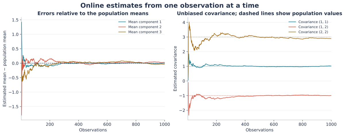

The companion notebook executes the Python example and checks it against the full-data calculation. Weighted observations will require a different denominator, as we will see next, but the scatter argument itself survives almost unchanged: every \(n\) becomes a weight sum and every residual acquires a weight in front of it.
Source: thesis Appendix B.2.1, specialized to unit weights and batch size one.
References
- Machine Learning and Deep Learning Approaches for Multivariate Time Series Prediction and Anomaly DetectionLeiden University, 2022
Enjoy Reading This Article?
Here are some more articles you might like to read next:
- Google Gemini updates: Flash 1.5, Gemma 2 and Project Astra
- Displaying External Posts on Your al-folio Blog
- Constructing a Linear Classifier from Known Decision-Boundary Points
- Binary Circles, Hamiltonian Cycles and de Bruijn Sequences
- Almost-Equal Isosceles Triangles: When Height Nearly Matches Base
- Online Estimation: Updating the Inverse Covariance Matrix
- Building Intelligent Agents for Connect-4: Final Considerations
- Online Estimation: The Memory of an Exponentially Weighted Estimator
- Building Intelligent Agents for Connect-4: Verification and Benchmarking
- Online Estimation: The Covariance of a Weighted Mean