Online Estimation: The Memory of an Exponentially Weighted Estimator
This post is the 6th part of a series of 7 articles:
- Online Estimation: Learning from a Changing Data Stream
- Online Estimation: The Mean and the Covariance Matrix
- Online Estimation: Weighted Observations and Mini-Batches
- Online Estimation: Exponential Forgetting
- Online Estimation: The Covariance of a Weighted Mean
- Online Estimation: The Memory of an Exponentially Weighted Estimator
- Online Estimation: Updating the Inverse Covariance Matrix
Because of its exponentially decaying weights, the estimator of the previous two articles has a limited historical memory: older observations fade out further with every new data point. This is what makes it possible to track a drifting distribution, and it costs accuracy when the data generating process is in fact stationary. Concretely, for \(\lambda<1\) the covariances of the estimated mean do not converge to zero as the sample grows. Some fixed amount of noise always remains, and how much depends on the rate of forgetting.
Appendix B.2.4 of my thesis (Thill, 2022) makes this precise by asking a single question: for which sample size \(n_{\mathrm{mem}}\) would an ordinary unweighted mean have the same covariance as our weighted one? The answer is short once the previous article’s result is available, and the derivation below follows the appendix line by line. What needs more care than the algebra is the interpretation, and I have narrowed the claim relative to the thesis, which invokes the central limit theorem at this point and concludes rather more than the calculation supports.
An Attractive Wrong Guess
For online exponential weights \(w'_i=\lambda^{n-i}\), the normalization factor is a geometric sum,
\[W_n=\sum_{i=1}^n w'_i=\sum_{i=1}^n\lambda^{n-i}=\frac{1-\lambda^n}{1-\lambda},\]which for \(\lambda<1\) converges towards a fixed value,
\[\lim_{n\to\infty}W_n=\lim_{n\to\infty}\frac{1-\lambda^n}{1-\lambda}=\frac{1}{1-\lambda}.\]At \(\lambda=0.99\) this limit is 100, and it is very tempting to conclude that \(n_{\mathrm{mem}}=W_n=100\). A small simulation refutes the guess directly: the distribution of the weighted means is visibly narrower than the distribution of ordinary means computed from 100 observations, so the memory must be larger than the weight sum suggests.

There is a second and rather more convincing reason why the weight sum cannot be the right quantity. Multiplying every unnormalized weight by the same constant changes \(W_n\) while leaving the mean completely unchanged, and any meaningful measure of the mean’s uncertainty must be invariant to that rescaling. The sum of weights is not, whereas the quantity we are about to derive is.
Deriving the Finite-Sample Memory
The previous article established that independent observations with common covariance \(\boldsymbol{\Sigma}\) and fixed normalized weights satisfy
\[\operatorname{Cov}(\bar{\mathbf{X}}_n)=\boldsymbol{\Sigma}\sum_{i=1}^nw_i^2,\]while an ordinary mean of \(n_{\mathrm{mem}}\) such observations has covariance \(\boldsymbol{\Sigma}/n_{\mathrm{mem}}\). Setting the two equal,
\[\boldsymbol{\Sigma}\frac{1}{n_{\mathrm{mem}}}=\boldsymbol{\Sigma}\sum_{i=1}^nw_i^2,\]the common covariance matrix cancels from both sides, leaving a purely scalar correspondence:
\[\begin{equation} n_{\mathrm{mem}}=\frac{1}{\sum_{i=1}^nw_i^2}=\frac{W_n^2}{W_n^{(2)}}. \label{eq:effective-n} \end{equation}\]This number need not be an integer, since it expresses a variance-equivalent sample size rather than a count of anything, and for positive weights it lies between one and the number of positively weighted observations. It is also invariant to rescaling all the weights, as required.
To evaluate \eqref{eq:effective-n} for exponential weights we expand the squared normalized weights and pull the constant normalization out of the sum:
\[\begin{aligned} \sum_{i=1}^nw_i^2 &=\sum_{i=1}^n\left(\frac{\lambda^{n-i}}{W_n}\right)^2 =\sum_{i=1}^n\frac{\big(\lambda^{n-i}\big)^2}{W_n^2}\\ &=\sum_{i=1}^n\frac{\lambda^{2(n-i)}}{\left(\sum_{i=1}^n\lambda^{n-i}\right)^2} =\sum_{i=1}^n\frac{\lambda^{2(n-i)}}{\left(\frac{1-\lambda^n}{1-\lambda}\right)^2}\\ &=\left(\frac{1-\lambda}{1-\lambda^n}\right)^2\sum_{i=1}^n\lambda^{2(n-i)}\\ &=\left(\frac{1-\lambda}{1-\lambda^n}\right)^2\frac{1-\lambda^{2n}}{1-\lambda^2}, \end{aligned}\]the last step being a second geometric sum, this time in \(\lambda^2\). For \(0<\lambda<1\) and large \(n\) both \(\lambda^n\) and \(\lambda^{2n}\) vanish, so
\[\lim_{n\to\infty}\sum_{i=1}^nw_i^2 =\lim_{n\to\infty}\left(\frac{1-\lambda}{1-\lambda^n}\right)^2\frac{1-\lambda^{2n}}{1-\lambda^2} =\frac{(1-\lambda)^2}{1-\lambda^2}.\]Taking the reciprocal of the finite-sample expression gives
\[\begin{aligned} n_{\mathrm{mem}}(n) &=\left(\frac{1-\lambda^n}{1-\lambda}\right)^2\frac{1-\lambda^2}{1-\lambda^{2n}}\\ &=\frac{(1-\lambda^n)^2}{(1-\lambda)^2}\cdot\frac{(1-\lambda)(1+\lambda)}{(1-\lambda^n)(1+\lambda^n)} =\frac{1+\lambda}{1-\lambda}\cdot\frac{1-\lambda^n}{1+\lambda^n}, \end{aligned}\]where both differences of squares have been factored. The second form is the more useful one, because the first factor is the limit and the second is a correction which approaches one. Taking the limit directly and clearing the quotient the same way,
\[\begin{aligned} \lim_{n\to\infty}n_{\mathrm{mem}}(n) &=\frac{1-\lambda^2}{(1-\lambda)^2} =\frac{1-\lambda^2}{(1-\lambda)^2}\cdot\frac{1+\lambda}{1+\lambda}\\ &=\frac{1+\lambda}{1-\lambda}\cdot\frac{1-\lambda^2}{(1+\lambda)(1-\lambda)} =\frac{1+\lambda}{1-\lambda}\cdot\frac{1-\lambda^2}{1-\lambda^2}, \end{aligned}\]so that
\[\begin{equation} n_{\mathrm{mem}}\longrightarrow\frac{1+\lambda}{1-\lambda}. \label{eq:memory-limit} \end{equation}\]At \(\lambda=0.99\) the limit is 199 rather than 100, which is roughly twice the weight sum and explains the mismatch in the simulation above. At \(\lambda=1\) one should use the equal-weight result \(n_{\mathrm{mem}}=n\) directly, since the closed forms here were derived under \(\lambda<1\) and substituting \(\lambda=1\) produces a quotient with a zero denominator. As \(\lambda\) tends to zero the estimator approaches a mean based on the newest observation alone.
Revisiting the Experiment

The thesis illustrates the same result with a density comparison using uniform observations, drawn from \(10^4\) samples. That is a genuinely different simulation from these Gaussian figures, which use a multivariate normal and many more replicates, and neither should be presented as the output of the other. Its close visual agreement is an illustration rather than a proof of identical distributions for general non-Gaussian inputs.
The Python notebook retains the two-stage comparison and adds the finite-sample prediction:
import numpy as np

lam, n = .99, 500
raw = lam**np.arange(n-1, -1, -1)
weights = raw/raw.sum()
effective_n = 1/(weights @ weights)
limit = (1+lam)/(1-lam)
print(effective_n, limit)  # approximately 196.402 and 199

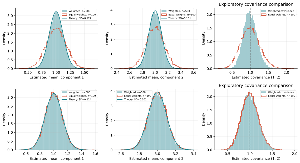
For a population variance of 3, the mean’s theoretical variance is about 0.015275 while the seeded simulation gives about 0.015189, and the difference is ordinary Monte Carlo variation. Note that after 500 observations the finite-sample memory is 196.402 rather than the limiting 199, so the 199-observation comparison is close but not exactly matched, and one should not expect the two histograms to coincide perfectly.
Mini-Batch Memory and Choosing a Decay
For equal-sized batches with unit weights within each batch, the fourth article gave
\[W_n=\mu\frac{1-\lambda^M}{1-\lambda},\qquad W_n^{(2)}=\mu\frac{1-\lambda^{2M}}{1-\lambda^2},\]so that \eqref{eq:effective-n} yields
\[n_{\mathrm{mem}}(M)=\frac{W_n^2}{W_n^{(2)}} =\frac{\mu^2\frac{(1-\lambda^M)^2}{(1-\lambda)^2}}{\mu\frac{1-\lambda^{2M}}{1-\lambda^2}} =\mu\frac{1+\lambda}{1-\lambda}\frac{1-\lambda^M}{1+\lambda^M} \quad\longrightarrow\quad \mu\frac{1+\lambda}{1-\lambda},\]by the same factoring as before. The extra factor \(\mu\) is precisely what explains why applying the same decay per batch and per observation gives different memory when measured in observations. For variable batch sizes or arbitrary incoming weights this fixed-batch expression no longer applies, and one should simply compute \(W_n^2/W_n^{(2)}\) from the actual accumulated sums, which the implementation maintains anyway.
If a target limiting online memory is \(L>1\), then solving \(L=(1+\lambda)/(1-\lambda)\) gives \(\lambda=(L-1)/(L+1)\). This is a useful parameterization under the IID comparison, and rather more intuitive than choosing \(\lambda\) directly, but it does not determine adaptation speed or uncertainty on every real time series. Weight half-life is another quantity sometimes quoted for the same purpose, and it measures something else again: how many updates reduce an individual weight by half.
What the Memory Interpretation Establishes
The derivation above matches one specific thing, namely the covariance of the estimated mean, and it does so under IID sampling with deterministic weights. For Gaussian observations that is enough to match the full distributions, since weighted and ordinary means are then both exactly Gaussian and a Gaussian is determined by its first two moments, provided the comparison sample size happens to be an admissible integer. For non-Gaussian inputs the derivation matches second moments and nothing more. The thesis reaches the same formula by way of the central limit theorem, which gives an asymptotic approximation after standardization rather than an exact finite-sample distribution, and under fixed forgetting the largest normalized weight does not vanish as the stream lengthens, so that route does not become exact by taking \(n\) large either.
Two further qualifications are worth stating plainly. Fixed forgetting leaves nonzero variability in the estimated mean even as more and more stationary observations arrive, which is the price of being able to adapt at all. And the exponential estimator is not an exact sliding window: older observations retain nonzero weights, its response to drift differs from a window’s response, and the sampling distribution of the covariance estimator needs separate analysis which \eqref{eq:memory-limit} does not provide, even though the mean and the scatter share a forgetting factor. Temporal correlation adds the cross-index covariance terms discussed in the previous article, and those do not vanish merely because the weights are well chosen.
The companion notebook contains the full simulation. Having established how weights affect the estimates and how to interpret them, the final article turns to maintaining an inverse covariance efficiently.
Source: thesis Appendix B.2.4 and Figure B.1. The memory is defined here as the sample size of an ordinary mean with the same covariance, and the normality and window-equivalence claims are qualified accordingly.
References
- Machine Learning and Deep Learning Approaches for Multivariate Time Series Prediction and Anomaly DetectionLeiden University, 2022
Enjoy Reading This Article?
Here are some more articles you might like to read next:
- Google Gemini updates: Flash 1.5, Gemma 2 and Project Astra
- Displaying External Posts on Your al-folio Blog
- Constructing a Linear Classifier from Known Decision-Boundary Points
- Binary Circles, Hamiltonian Cycles and de Bruijn Sequences
- Almost-Equal Isosceles Triangles: When Height Nearly Matches Base
- Online Estimation: Updating the Inverse Covariance Matrix
- Building Intelligent Agents for Connect-4: Final Considerations
- Building Intelligent Agents for Connect-4: Verification and Benchmarking
- Online Estimation: The Covariance of a Weighted Mean
- The Hexadecimal Digit Canon Challenge: Solution